[From
Bjorn Simonsen (2004.02.18.15:00 EuST)]
[From Rick Marken (2004.02.04.1025)]
Ø
The result
shows what appears to be a clear positive relationship between
discount
Ø
rate and inflation rate, exactly the opposite of the relationship
assumed in popular
Ø
discussions of economic policy.
To the right you see the graph from
Norwegian data.
[insert
inflatedisc.jpg here]
The positive
relationship between discount rate and inflation rate shows up at nearly
all phase delays between
these time plots of these two variables. This is shown in the
lagged analysis in the
attached laginflatedisc.jpg. The lags/leads on the X axis are the
number of months by
which the discount rate leads (- values) or lags (+ values) inflation
rate. Discount rate
does not become negatively related to inflation until 22 months before
the inflation changes.
And the negative relationship is quite low. The negative relationship
between discount rate
and inflation never exceeds -.11, and that that level of negative
relationship doesn’t
occur until discount rate leads inflation by 36 months (3 years).
Compare this to the
very strong positive relationship (.59) between discount and inflation
rate that reaches a
maximum when discount rate follows inflation rate within 11 months.
Thank you for your answer in private mail
2004.02.11. I have till now spent some time on this thread and I will give you
some comments. I have collected the same data as you did and I have analysed
them in your way.
I don’t agree completely with your
formula “ ((CPI(t)-CPI(t-1))/CPI(t).) is the way the government
measures inflation rate”. I think divisor shall be CPI(t-1), because the change
is from time (t-1). And the formula
((CPI(t)-CPI(t-1))/CPI(t-1)). I thought that this should give growth
when you have decrease and reversed, but I can’t see any differences in my
graphs in contrast to yours. Maybe you have used ((CPI(t)-CPI(t-1))/CPI(t-1))
when you calculated yourself?
Here is
my graph where I show the Correlation coefficients phase leaded/lagged. It is Quite as yours.

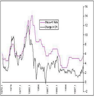
image003.wmz (4.27 KB)
image005.wmz (2.07 KB)
image007.wmz (1.56 KB)
image009.wmz (2.23 KB)
image011.wmz (1.28 KB)
image013.wmz (6.28 KB)
image015.wmz (4.36 KB)
image017.wmz (4.37 KB)
oledata2.mso (305 KB)
···
To
the left you find my graph from US data. The graph is quite like yours of
course. To the right you see a different graph. Here is no negative data at
all.
Ø
………This results in the positive correlation between
discount and feedback when
Ø
discount follows inflation (positive lag values). But changes
in the discount rate seem
Ø
to be positively related to inflation (rather than
negatively, as assumed by the Fed) as
Ø
indicated by the positive relationship between
discount and inflation when discount
Ø
precedes inflation (negative lag values). This
positive feedback relationship between
Ø
the Fed chief’s actions and the results of those
actions on the controlled variable
Ø
inflation – would result in runaway inflation
if the Fed chie kept raising rates. But
Ø
the positive relationship between the Fed chief
actions and inflation seems to level
Ø
off after a few months. So runaway inflation is
prevented by the limit to the Fed chief
Ø
response to the inflation he has coaused causes by his
own actions.
I
think there is a positive
correlation between Discount
and the Inflation rate when the Discount is correlated with the Inflation rate some months before. But
the value is low, and it doesn’t tell us much.
Also I see the positive feedback between
the Discount and the effect on inflation and I think the Fed chief has
something to learn about negative feedback.
Ø
Increases in the Fed discount rate takes money out of
the economy, which should make
Ø
it difficult to get money for investment and growth.
My own visual inspection of the data
Ø
led me to the same conclusion: it looks like discount
rate and growth are negatively
Ø
related. But I wanted a quantitative measure so I got
the raw data and made my
Ø
own version of Canterbury’s Figure 14.2, which is the
graph is seen in growdisc.jpg.
Ø
I used the raw data (actually, I was able to get data
that went back to 1959, rather
Ø
than just 1975, but the statistical results are the
same for the 1959-2000 and for the
Ø
1975-2000 time period) to compute the actual
correlation between discount rate and
Ø
growth. And the results were a big surprise. It turns
out that the zero lagged correlation
Ø
between discount and growth is positive (.25). The
apparent negative relationship
Ø
between the discount and growth curves seen in
growdisc.jpg is actually an optical
Ø
illusion. The complete phase analysis of the
relationship between discount and growth
Ø
is shown in the graph in laggrowthdisc.jpg.
I did the same analyse as you and my graph
is quite like your laggrowthdisc.jpg. Below my graph.
But
my graph presents the Correlation coefficient for different Phase lags/leads
some different from your laggrowthdisc.jpg. My graph is below.
I
have tried to reanalyse my calculations and I shall do it again. I have used
the formula 100*(C21-C20)/C20 in Excel where the date in row 20 is lower than
the date in row 22.
But
both graphs indicate that
Ø
What this analysis shows is that changes in discount
rate that precede growth are
Ø
actually positively related to growth, a result that
is, again, completely the opposite
Ø
of what many economic policy experts seem to believe
is true. Increases in discount
Ø
rate are believed to lead to decreased growth. This
would show up as a negative
Ø
relationship between discount rate and growth when
discount rate precedes growth.
Ø
In fact, just the opposite is seen.
Yes
Ø
All the results presented here describe relationships
between variables that exist as
Ø
part of a closed loop system. I think the only way to
figure out what is actually going
Ø
on – that is, to figure out how variables like
discount rate, grwoth and inflation actually
Ø
influence each other – is to build closed loop models
and try to match the behavior of
Ø
the models (over time) to the observed behavior of the
variables observed.
I
have done it and I am a little excited.
I
used your model in [From Rick Marken (2004.02.07.2330)]
p = Discount in preceding month-Actual inflation rate in the preceding
month
Discount = Discount + 0.1 * ((0.01 * (0-p)) - Discount) *dt, where dt =1
month
Here you can see the graph showing the Inflation rate (upper graph) and
the Simulated Discount (lower graph)
I calculated the
Correlation coefficient between the data for same date, and it was 0.49. Then I
calculated a Correlation coefficient between the Inflation rate and the
Simulated Discount, the inflation rate for one month earlier than the Simulated
Discount setting. Here the
Correlation coefficient is 1,00. I guess you don’t believe it. Therefore I give
you a part of my calculations
I used the
formula output = output + 0.01 * (8 * (-p) -
output)
You used the
formula p = sim_discount (i-lag) -
dCPI (i-lag)
I used the
formula p = sim_discount - dCPI (i-lag)
CPI
Date
dCPI Simulated Discount
39,8
1970.12
0,50505051
0,45094052
39,8
1971.01
0
0,44866304
39,9
1971.02
0,25125628
1,5231E-07
40
1971.03
0,25062657
0,2232043
40,1
1971.04
0,25
0,2226449
40,3
1971.05
0,49875312
0,22208828
40,6
1971.06
0,74441687
0,44306874
40,7
1971.07
0,24630542
0,66130476
40,8
1971.08
0,24570025
0,21880619
40,8
1971.09
0
0,21826859
40,9
1971.10
0,24509804
1,5231E-07
40,9
1971.11
0
0,21773361
41,1
1971.12
0,48899756
1,5231E-07
The dCPI is calculated
as (A35-A34)/A34 ex. Line 3 an 4 (40-39.9)/39.9 = 0.25062657
And at line 4 I have
calculated the Simulated Discount as D35+0.001*(0.25*(0-(D34-C34))-D35). Here
the Correlation coefficient taken at the same date is 0.08. But if you Phase
displace one month the dCPI and the Simulated Discount 1 month later you get a
Correlation coefficient at 1.00. Try it.
I have worked with a
simulated Discount using your formula “output = output + 0.01 * (8 * (-p) -
output)” on Norwegian data. The graph below shows the Norwegian Inflation rate
and a Simulated Discount.
I calculated the
Correlation coefficient between the data for same date, and it was 0.20. Then I
calculated a Correlation coefficient between the Inflation rate and the
Simulated Discount, the inflation rate for one month earlier than the Simulated
Discount setting. Here the
Correlation coefficient is 1,00. I guess you don’t believe it. Therefore I give
you a part of my calculations
Here I used the same
formula you used output = output + 0.01 * (8 * (-p) -
output)
CPI
Date
dCPI Discount Change of Simulated Change of the Discount
The Discount
64,5
1986M03
0,78125
13,37
-1,32841328
0,278648555
64,9
1986M04
0,62015504
13,65
2,09424084
0,694444444
65
1986M05
0,1540832
14,36
5,2014652
0,551248923
66,1
1986M06
1,69230769
14,31
-0,34818942
0,136962849
66,8
1986M07
1,05900151
14,58
1,88679245
1,504273504
67
1986M08
0,2994012
14,56
-0,13717421
0,941334678
68
1986M09
1,49253731
14,46
-0,68681319
0,266134398
68,3
1986M10
0,44117647
14,6
0,96818811
1,326699834
68,5
1986M11
0,29282577
15,02
2,87671233
0,392156863
68,8
1986M12
0,4379562
16,4
9,18774967
0,260289572
69,8
1987M01
1,45348837
16,34
-0,36585366
0,389294404
70,5
1987M02
1,00286533
15,09
-7,6499388
1,291989664
The dCPI is calculated
as (A35-A34)/A34 ex. Line 4 an 5 (40-39.9)/39.9 = 0.25062657
And at line 5 I have
calculated the Simulated Discount as F20+0.01*(8*(0-(F20-C19))-F20). Here the
Correlation coefficient taken at the same date is 0.00. But if you Phase
displace one month, the dCPI and the Simulated Discount 1 month later, you get
a Correlation coefficient at 1.00. Try it.
I will show you a wonderful
figure from my Norwegian data.
This is how the
Norwegian Bank (Norwegian FED) would like to see the graph of the Inflation
rate and the Change of Discount.
The Correlation
coefficient with 1-month phase shift is –1.00, telling me that their action with the discount is exact
opposite the Inflation rate. When the inflation rate grows they choose a
Discount with correct effect.
I don’t believe this
is true. I have tried to extricate myself and find where I do something wrong. But
I don’t find it. So I am asking for comments.
Have a nice weekend.
bjorn