refer you to two of several messages from about a year ago. In case
you haven’t been keeping your own archive of CSGnet messages for
that long, I copy the main body of the messages here, despite their
length. The first was after quite a long thread on the topic, rife
with misunderstandings about the nature of information as Shannon
described it. The second was intended as part of a tutorial series
on information theory, in part to dispel these misunderstandings. I
think these two should be enough to be getting on with.
Martin
···
[Philip
2014.01.29.08.00]
Let me see yours and mr Kenway's work concerning information
theory. Mine will soon follow (Ive been working on it everyday).
[Martin Taylor
2012.12.08.11.32]
[From
Bruce Abbott (2012.12.07.1830 EST)]
Rick Marken
(2012.12.07.1150)] –
One
of us is confused here – and I don’t think it’s me! (nor
Martin)
Martin Taylor (2012.12.06.23.52)
MT:... Somehow, the information
from the disturbance appears at the output, and the
only path through which this can happen is by way of
the internal circuitry of the control system.
RM: You are assuming that the only way for information
about the disturbance to appear at the output is for
this information to have gone through the organism.
How
else could it get there? Magic?
This is just a fancy way of saying
that the causal (S-R) model of behavior must be true.
Not
so. It’s a circular loop of causality, but each
element within the loop transmits information only one
way, from CV to perceptual signal to error signal to
output and back to CV. And because of loop delay,
these effects do not propagate instantly and
simultaneously around the loop.
Let's see if we can take a different tack to make it more
intuitively easy to see how information from the disturbance gets
to the output even though the input quantity – the controlled
environmental variable – is influenced by both the disturbance
and the output of the control system. I’ll borrow from the usual
way differential calculus is introduced, by treating a smooth
waveform as though it was created by making a number of step
changes, and reducing the time between changes so they become
indefinitely small. But first, I want to illustrate how control
can be seen as measurement.
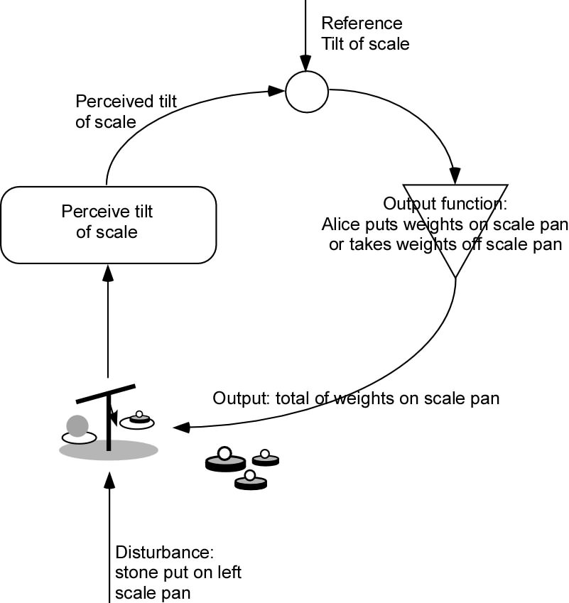
To see why control can be considered to be measurement, think of
this example. Alice wants to know how heavy is a stone she has
picked up. She has a balance scale and a set of weights weighing
2, 1, 1/2, 1/4 … kilos. She puts the stone on one pan, and the
scale tilts down to the side on which she put the stone, so she
puts a weight on the other pan. The tilt stays the same, so she
adds another weight and the scale tilts the other way. Alice
removes the last weight she added and adds the next lighter one.
She keeps adding and removing weights until the scale stays level
or she runs out of ever smaller weights.
What is Alice doing? Alice is performing the actions of the output
function of a control loop, looking at the error that is shown by
the tilt of the scale, and altering her output (the weights on the
other pan) until the error is zero. The output, which is the sum
of the weights in the other pan, now is a measure of the weight
of Alice’s stone in exactly the same way that the output of any
control system measures the disturbance to its controlled
environmental variable.
Of course, there need be no human Alice in this story. The
perceptual function signals only the direction in which the scales
tilt, so the error is only a binary value, which could be called
“1” or “0”, “left” or “right”, “too heavy” or “too light”, or any
other contrasting labels. I will call the values “left” and
“right” according to which side of the scale is heavier. Likewise,
there is no need for Alice to provide the output function. It
could be a mechanical device that is provided with the weights
that have values in powers of two times 1 kilo, with 2 kilos the
heaviest. We can assume that the scale would break if the stone
was over 4 kilos!
The output device would load and unload these weights onto and off
the scale pan according to the following algorithm. The stone is
on the left pan.
1. Add to the right-hand pan the heaviest weight not yet tried
(initially, since none have been tried, that means the 2 kilo
weight).
  2. If all the available weights have been tried, stop. Else...

  3a. If the error is "left" go to step 1 (there is not enough
weight in the right hand pan)
3b, if the error is "right", remove the lightest weight in the pan
and add the heaviest weight not yet tried.
At the end of this process, the balance is as close as the machine
(or Alice) can make it using the available weights. Anyone who
wanted to know the weight of the stone could simply read out the
weights in the pan as a binary number of kilos, with the units
starting at the 2 kilo weight. Those weights are the current
output value of the control system., which, without Alice, is a
perfectly standard control loop.
One could continue this example using a continuously varying
weight instead of the stone, but I think it is better to talk
about the general case of an idealized control system with no
noise and no transport lag. Transport lag introduces an
independent limit on the quality of control, a limit that has
already been mentioned in this complex of threads. It also
introduces some complication in the other computations,
complication that is unnecessary in this illustrative discussion.
We consider the "basic-standard" control system that has a pure
integrator as its output function.
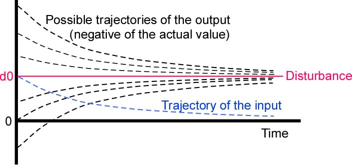
First, let's treat the effect of one step change in the
disturbance value. We assume that the error is initially zero, and
at time t0 the disturbance suddenly goes from whatever value it
may have had previously to d0. We treat this single step, and then
consider the effects of a series of steps. We start by showing how
the integrator rate parameter controls how fast information about
the disturbance arrives at the output – how fast the control
system measures the disturbance value.
Let us trace the signal values at various places in the loop as
time passes after the step at time t0. At time t0+e (e means
epsilon, an indefinitely small amount), the error value is -d and
the output value qo is zero. At this early time the output value
is whatever it was before the step, and has an unchanged influence
on the value of the input quantity qi. As time passes, the output
value changes exponentially until after infinite time it reaches
-d. Assuming q0 was initially zero, then at time t:
  qo(t) = -d0*(1-e^(-G*(t-t0))).

  At the same time, the input value qi approaches zero by the same
exponential:
  qi(t) = 1 - e^(-G*(t-t0))

  Exponential changes in value are quite interesting in information
theory, as they often indicate a constant bit rate of information
transfer. To see this, you must understand that although the
absolute uncertainty about the value of a continuous variable
either before or after a measurement or observation is always
infinity, the information gained through the measurement or
observation is finite. If the range of uncertainty about the value
(such as standard deviation of measurement) is r0 before the
measure and r1 after the measure, the information gained is
log2(r0/r1) bits.
Measurements and observations are never infinitely precise. When
someone says their perception is subjectively noise-free and
precise, they nevertheless would be unable to tell by eye if an
object changed location by a nanometer or declined in brightness
by one part in a billion. There is always some limit to the
resolution of any observation, so the issue of there being an
infinite uncertainty about the value of a continuous variable is
never a problem. In any case in which a problem of infinite
uncertainty might seem to be presenting itself, the solution is
usually to look at the problem from a different angle, but if that
is not possible it is always possible to presume a resolution
limit, a limit that might be several orders of magnitude more
precise than any physically realizable limit, but a limit
nevertheless.
(If you want to get a more accurate statement, and see the
derivation of all this, I suggest you get Shannon’s book from
Amazon at the link I provided earlier
).
In the above example, q0 could have started at any value whatever,
and would still have approached -d exponentially with the same
time constant. The output value qo has the character of a
continuous measurement of the value of the disturbance, and this
measurement gains precision at a rate given by e^(-G*(t-t0)). (The
units of G are 1/seconds).
What is this rate of gain in precision, in bits/sec? One bit of
information has been gained when the uncertainty about the value
of d0 has been halved. In other words, the output has gained one
bit of information about the disturbance by the time tx such that
e^(-G*(tx-t0)) = 0.5
Taking logarithms (base 2) of both sides, we have
log2(e)(-G(tx-t0)) = -1
tx-t0 = 1/(Glog2(e)) = 1/(G1.443…) seconds
That is the time it takes for q0 to halve its distance to its
final value -d0 no matter what its starting value might have been,
which means it has gained one bit of information about the value
of the disturbance. The bit rate is therefore G1.443… bits/sec.
That is the rate at which the output quantity q0 gains information
about the disturbance, and also is the rate at which the input
quantity loses information about the disturbance. The input
quantity must lose information about the disturbance, because it
always approaches the reference value, no matter what the value of
the disturbance step. I suppose you could look upon G1.443 as the bit rate of the loop
considered as a communication channel, but it is probably not
helpful do do so, as the communication is from the input quantity
back to itself. Without the complete loop, q0 does not act as a
measure of d0, but continues negatively increasing linearly
without limit at a rate Gd0. It is better just to think of
G1.443 as the rate at which information from the disturbance
appears at the output quantity.
As a further matter of clarification, I suppose we ought to
mention the behavioural illusion here. If the environmental
feedback path is not a simple connector with a gain of unity, the
output quantity differs from the disturbance value. The mismatch
does not affect the information relationship between the
disturbance and the output quantity, since the environmental
feedback path provides a single-valued environmental feedback
function. It is always possible to compute the influence of the
output on the input quantity if you know the output value q0. This
means that q0 and the influence of the output on the input
quantity are informationally identical, whatever their functional
relationship, providing the environmental feedback function does
not change. If it does change, the effect is similar to adding a
noise source to a communication channel, a situation that was
Shannon’s primary concern and provides no particular complication
to the analysis. (Or in the case of Marken’s demo that involves
switching the sense of the environmental feedback path, the
communication analogy is the band-switching secret communication
procedure patented by the movie star Hedy Lamarr; in both cases,
the switching must be separately detected or otherwise known).
As a specific example, if the environmental feedback path has a
gain of 2, the output quantity will converge to a value of d/2.
The convergence to d/2 is at the same exponential rate as would
have been the case for en environmental feedback path gain of 1.0,
providing an information gain rate that is determined only by the
integration rate parameter G. Information from the disturbance
still arrives at the output quantity (and is lost from the input
quantity) at a rate G1.443… From now on, we will give the label “T” to the rate at which the
output gains information about the disturbance. T = G1.443… bits/sec.
The rate of information gain about the disturbance value at the
output quantity is independent of the disturbance waveform and of
the environmental feedback function. It is a property of the
internal circuitry of the control system. Accordingly, we can make
some estimates about the achievable precision of control for
disturbances that are not simple step functions. First, however,
we should look at the effect of a second and subsequent step
change in the disturbance value.
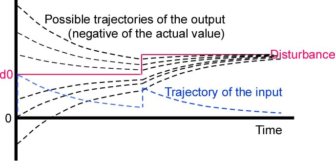
The disturbance value changed abruptly to d0 at time t0. Now at
time t1 the disturbance value jumps to d1. The input quantity adds
d1-d0 to whatever value it had arrived at by t1. The error value
jumps by the same amount, but the output value qo does not change
immediately, because of the integrator output function. It starts
changing exponentially toward (the negative of) the new value of
the disturbance.
At t1+e, the output quantity has a value that is unknown, because
ever since t0 it has been in the process of approaching -d0
exponentially from some unknown starting point. The uncertainty of
its current value is T*(t1-t0) bits less than it had been at time
t0, because it was performing a process functionally equivalent to
measuring the value d0. Now it has to start forgetting the value
d0 and start measuring the value d1. Less colloquially, the mutual
information between the output quantity and the disturbance value
is instantly decreased by the uncertainty of the change in
disturbance value, while the mutual information between the
disturbance value and the input value is increased by the same
amount.
By how much are the mutual information values changed by the new
step? Since the absolute uncertainty of a continuous variable is
infinite, can that change be measured? Shannon shows again that it
can. The amount is log2(r_new/r_old) where r_new is the new range
of uncertainty (such as standard deviation) and r_old is the old
range of uncertainty. The new range of uncertainty depends on the
probability distribution of values that can be taken by the
disturbance at that time, which may be unknown. It is not a new
unknown, however, since the original disturbance step came from
the same distribution, and the original value of the output
quantity probably came from the same distribution (modified, of
course, by the inverse of the environmental feedback function) if
the system had been controlling prior to the first step that we
analyzed.
After the second step change in the disturbance value, the output
quantity is gaining information, still about the disturbance
value, but not about d0. Now it is gaining information about d1
and losing information about d0. At the same time, the input
quantity is losing information about d1, as well as about any
remanent information about d0 that might still have been there at
time t1. All this is happening at a rate of T = G*1.44.3…
bits/sec.
The effects of third and subsequent steps in the value of the
disturbance are the same. The output continues to gain information
about the most recent value of the disturbance at T bits/sec while
losing information about prior values at the same rate, and while
the input also loses information about the new and old values at T
bits/sec. Making the steps smaller and closer in time, we can
approximate a smooth waveform with any desired degree of
precision. No matter what the disturbance waveform, the output is
still getting information about its value at T bits/sec, and
losing information about its history at the same rate. So long as the disturbance variation produces less than T
bits/sec, control is possible, but if the disturbance variation is
greater than T bits/sec, control is lost. The spike in the input
value at a step change in the disturbance is an example of that,
where control is completely lost at the moment of the step, and
gradually regained in the period when the disturbance remains
steady, not generating uncertainty.
This is getting rather too long for a single message, so I will
stop there. I hope it explains just how information gets from the
disturbance to the output, and how fast it does so in the case of
the ideal noiseless control system with no lag and a pure
integrator output function.
Martin
http://www.amazon.com/Mathematical-Theory-Communication-Claude-Shannon/dp/0252725484/ref=sr_1_1?s=books&ie=UTF8&qid=1354736909&sr=1-1&keywords=Shannon%2C+C.+E.
[Martin Taylor
2013.01.01.12.40]
As you can see by the date stamp, I started this on New
Year’s Day, expecting it to be quite short and to be
finished that day. I was wrong on both counts.
This message is a follow-up to [Martin Taylor
2012.12.08.11.32] and the precursor of what I hope will be
messages more suited to Richard Kennaway’s wish for a
mathematical discussion of information in control. It is
intended as part 1 of 2. Part 1 deals with the concepts and
algebra of uncertainty, information, and mutual information.
Part 2 applies the concepts to control.
Since writing [Martin Taylor 2012.12.08.11.32], which showed
the close link between control and measurement, and followed
the information “flow” around the loop for a particular
control system, I have been trying to write a tutorial
message that would offer a mathematically accurate
description of the general case while being intuitively
clear about what is going on. Each of four rewrites from
scratch has become long, full of equations, and hardly
intuitive to anyone not well versed in information theory.
So now I am trying to separate the objectives. This message
attempts to make information-theoretic concepts more
intuitive with few equations beyond the basic ones that
provide definitions. It is nevertheless very long, but I
have avoided most equations in an attempt to make the
principles intelligible. I hope it can be easily followed,
and that it is worth reading carefully.
My hope is that introducing these concepts with no reference
to control will make it easier to follow the arguments in
later messages that will apply the concepts and the few
equations to control.
        This tutorial message has several sections, as follows:
        Basic background
           concepts
           definitions
              uncertainty
                  comments on "uncertainty"
              information
                  Information as change in uncertainty
                  mutual information
        Time and rate
           Uncertainty
           Information
           Information and history
        Some worked out example cases
           1. A sequence like "ababababa..."
           2. A sequence like "abacacabacababacab...."
           3. A sequence in which neighbour is likely to follow
neighbour
4. A perfect adder to which the successive input values
are independend
5. A perfect adder to which the successive input values
are not independent
6. Same as (5) except that there is a gap in the history
– the most recent N input samples are unknown.
[Because I don't know whether subscripts or Greek will come
out in everyone’s mail reader, I use “_i” for subscript “i”,
and Sum_i for “Sum over i”. "p(v)’ means “the probability of
v being the case”, so p(x_i) means "the probability X is in
state i"and p_x_i(v) means “the probability that v is the
case, given that x is in state i”, which can also be written
p(v|x_i).]
        ------------Basic equations and concepts: definitions-------

        1. "Probability" and "Uncertainty"

        In information theory analysis, "uncertainty" has a precise
meaning, which overlaps the everyday meaning in much the
same way as the meaning of “perception” in PCT overlaps the
everyday meaning of that word. In everyday language, one is
uncertain about something if one has some idea about its
possible states – for example the weather might be sunny,
cloudy, rainy, snowy, hot, … – but does not know in which
of these states the weather is, was, or will be now or at
some other time of interest. One may be uncertain about
which Pope Gregory instituted the Gregorian calendar, while
feeling it more likely that it was Gregory VII or VIII than
that it was Gregory I or II. One may be uncertain whether
tomorrow’s Dow will be up or down, while believing strongly
that one of these is more probable than that the market will
be closed because of some disaster.
If one knows nothing about the possibilities for the thing
in question (for example, “how high is the gelmorphyry of
the seventh frachillistator at the winter solstice?”) one
seldom thinks of oneself as “uncertain” about it. More
probably, one thinks of oneself as “ignorant” about it.
However, “ignorance” can be considered as one extreme of
uncertainty, with “certainty” as the other extreme.
“Ignorance” could be seen as “infinite uncertainty”, while
“certainty” is “zero uncertainty”. Neither extreme condition
is exactly true of anything we normally encounter, though
sometimes we can come pretty close.
Usually, when one is uncertain about something, one has an
idea which states are more likely to be the case and which
are unlikely. For example, next July 1 in Berlin the weather
is unlikely to be snowy, and likely to be hot, and it is
fairly likely to be wet. It is rather unlikely that the Pope
is secretly married. It is very likely that the Apollo
program landed men on the moon and brought them home. One
assigns relative probabilities to the different possible
states. These probabilities may not be numerically exact, or
consciously considered as numbers, but if you were asked if
you would take a 5:1 bet on it snowing in Berlin next July 1
(you pay $5 if it does snow and receive $1 if it doesn’t
snow), you would probably take the bet. If you would take
the bet, your probability for it to snow is below 0.2.
Whether "uncertainty" is subjective or objective depends on
how you treat probability. If you think of probability as a
limit of the proportion of times one thing happens out of
the number of times it might have happened, then for you,
uncertainty is likely to be an objective measure. I do not
accept that approach to probability, for many reasons on
which I will not waste space in this message. For me,
“probability” is a subjective measure, and is always
conditional on some other fact, so that there really is no
absolute probability of X being in state “i”.
Typically, for the kind of things of interest here, when the
frequentist “objective” version is applicable, the two
versions of probability converge to the same value or very
close to the same value. Indeed, subjective probability may
be quite strongly influenced by how often we experience one
outcome or another in what we take to be “the same”
conditions. In other cases, such as coin tossing, we may
never have actually counted how many heads or tails have
come up in our experience, but the shape of the coin and the
mechanics of tossing make it unlikely that either side will
predominate, so our subjective probability is likely to be
close to 0.5 for both “heads” and “tails”. As always, there
are conditionals: the coin is fair, the coin tosser is not
skilled in making it fall the way she wants, it does not
land and stay on edge, and so forth.
In order to understand the mathematics of information and
uncertainty, there is no need to go into the deep
philosophical issues that underlie the concept of
probability. All that is necessary is that however
probabilities are determined, if you have a set of mutually
exclusive states of something, and those states together
cover all the possible states, their probabilities must sum
to 1.0 exactly. Sometimes inclusivity is achieved by
including a state labelled “something else” or
“miscellaneous”, but this can be accommodated. If the states
form a continuum, as they would if you were to measure the
height of a person, probabilities are replaced by
probability density and the sum by an integral. The integral
over all possibilities must still sum to 1.0 exactly.
        -------definitions-----

        First, a couple of notations for the equations I do have to
use:
I use underbar to mean subscript, as in x_i for x subscript
i.
p(x_i) by itself means "Given what we know of X, this is the
probability for us that X is (was, will be) in state i" or,
if you are a frequentist, “Over the long term, the
proportion of the times that X will be (was) in state i is
p(x_i)”.
I mostly use capital letters (X) to represent systems of
possible states and the corresponding lower-case letters to
represent individual states (x for a particular but
unspecified state, x_i for the i’th state).
p(x_i|A) means "If A is true, then this is our probability
that X is in state i" or “Over the long term, when A is
true, the proportion of the time that X will be in state i
is p(x_i)”. In typeset text, sometimes this is notated in a
more awkward way, using A as a subscript, which I would have
to write as p_A(x_i).
I will not make any significant distinction between the
subjective and objective approaches to probability, but will
often use one or the other form of wording interchangeably
(such as “if we know the state of X, then …”, which you
can equally read as “If X is in a specific state, then
…”). Depending on which approach you like, “probability”,
and hence “uncertainty”, is either subjective or objective.
It is the reader’s choice.
I use three main capital letter symbols apart from the Xs
and Ys that represent different systems. U( ) means
“Uncertainty”, I( ) means Information, and M( : ) means
mutual information between whatever is symbolized on the two
sides of the colon mark. The parentheses should make it
clear when, say, “U” means a system U with states u_i and
when it means “Uncertainty”.
        -----definition of "uncertainty"----

        If there is a system X, which could be a variable, a
collection of possibilities, or the like, that can be in
distinguishable states x_i, with probabilities p(x_i), the
uncertainty of X is _defined _ by two formulae,
one applicable to discrete collections or variables
        U(X) = - Sum_i (p(x_i) log(p(x_i)))

        the other for the case in which "i" is a continuous
variable. If “i” is continuous, p(x_i) becomes a probability
density and the sum becomes an integral
        U(X) = - Integral_i (p(x_i) log(p(x_i)) di).

        That's it. No more, no less. Those two equations define
“uncertainty” in the discrete and the continuous case.
(Aside: Von Neumann persuaded Shannon to stop calling U(X)
“uncertainty” and to call it “Entropy” because the equations
are the same. This renaming was unfortunate, as it has
caused confusion between the concepts of uncertainty and
entropy ever since.)
If X is a continuous variable, the measure of uncertainty
depends on the choice of unit for “i”. If, for example, X
has a Gaussian distribution with standard deviation s, and
we write H for log(sqrt(2PIe)), the uncertainty of X is H
-
log(s). The standard deviation is measured in whatever
units are convenient, so the absolute measure of uncertainty
is undetermined. But whatever the unit of measure, if the
standard deviation is doubled, the uncertainty is increased
by 1 bit. Since we usually are concerned not with the
absolute uncertainty of a system, but with changes in
uncertainty as a consequence of some observation or event,
the calculations give well-defined results regardless of the
unit of measure. When the absolute uncertainty is of
interest, one convenient unit of measure is the resolution
limit of the measuring or observing instrument, since this
determines how much information can be obtained by
measurement or observation.
There are a few other technical issues with the uncertainty
of continuous variables, but calculations using uncertainty
work out pretty much the same whether the variable is
discrete or continuous. Unless it matters, in what follows I
will not distinguish between discrete and continuous
variables.
        --------comments on "uncertainty-----

        Why is Sum(p*log(p)) a natural measure of "uncertainty"?
Shannon, in his 1947 monograph that introduced information
theory to the wider world, proved that this is the only
function that satisfies three natural criteria:
(1) When the probabilities vary continuously, the
uncertainty should also vary continuously.
(2) The uncertainty should be a maximum when all the
possibilities are equally probable.
(3) If the set is partitioned into two subsets, the
uncertainty of the whole should be the weighted sum of the
uncertainties of the two parts, the weights being the total
probabilities of the individual parts. Saying this in the
form of an equation, if X has possibilities x_1, x_2, …
x_n and they are collected into two sets X1 and X2, then
U(X) = p(X1)*U(X1) + p(X2)*U(X2),
where p(Xk) is the sum of the probabilities of the
possibilities collected into set Xk.
One important consequence of the defining equation U(X) =
Sum_i(p(x_i)*log(p(x_i))) is that the uncertainty U(X) is
always positive and ranges between zero (when one of the
p(x_i) is 1.0 and the rest are zero) and log(N) (when there
are N equally probable states of X). The logarithm can be to
any base, but base 2 is conventionally used. When base 2 is
used, the uncertainty is measured in “bits”. The reason for
using base 2 is convenience. If you can determine the actual
state through a series of yes-no questions to which every
answer is equally likely to be yes or no, the uncertainty in
bits is given by the number of questions.
I will use the term "global uncertainty of X" for the case
when nothing is assumed or known about X other than its
long-term probability distribution over its possible states.
This is what is meant by “U(X)” in what follows, unless some
other conditional is specified in words.
In certain contexts, uncertainty is a conserved quantity.
For example, if X and Y are independent, the joint
uncertainty of X and Y, symbolised as U(X,Y), is
        U(X,Y) = U(X) + U(Y)

        where U(X,Y) is the uncertainty obtained from the defining
equation if each possible combination of X state and Y state
(x_i, y_j) is taken to be a state of the combined system.
The concept can be extended to any number of independent
variables:
        U(X, Y, Z, W....) = U(X) + U(Y) + U(Z) + U(W) +...

        Using the subjective approach to probability, "independent"
means “independent given what is so far known”. It is not
clear how the term can legitimately be used in a frequentist
sense, because any finite sample will show some apparent
relationships among the systems, even if an infinite set of
hypothetical trials would theoretically reduce the apparent
relationships to zero. A frequentist might say that there is
no mechanism that connects the two systems, which means they
must be independent. However, to take that into account is
to concede the subjectivist position, since the frequentist
is saying that as far as he knows , there is
no mechanism. Even if there was a mechanism, to consider it
would lead the frequentist into the subjectivist heresy.
Uncertainty is always "about" something. It involves the
probabilities of the different states of some system X, and
probabilities mean nothing from inside the system in
question. They are about X as seen from some other place or
time. To say this is equivalent to saying that all
probabilities are conditional. They depend on some kind of
prior assumption, and taking a viewpoint is one such
assumption.
Consider this example, to which I will return later: Joe
half expects that Bob will want a meeting, but does not know
when or where that is to be if it happens at all. What is
Joe’s uncertainty about the meeting?
Joe thinks it 50-50 that Bob will want a meeting. p(meeting)
= 0.5
If there is to be a meeting, Joe thinks it might be at Joe's
office or at Bob’s office, again with a 50-50 chance.
If there is to be a meeting, Joe expects it to be scheduled
for some exact hour, 10, 11, 2, or 3.
For Joe, these considerations lead to several mutually
exclusive possibilities:
        No meeting, p=0.5

        Bob's office, p = p(meeting)*p(Bob's office | meeting) =
0.5*0.5 = 0.25
Joe's office p = p(meeting)*p(Joe's office | meeting) =
0.5*0.5 = 0.25
Joe has 1 bit of uncertainty about whether there is to be a
meeting, and with probability 0.5, another bit about where
it is to be. Overall, his uncertainty about whether and
where the meeting is to be is
U(if, where) = -0.5log(0.5) - 2*(0.25log(0.25) = -0.5*(-1) -
0.5*(-2) = 1.5 bits
no meeting
meeting&&either office
Another way to get the same result is to use a pattern that
will turn up quite often
U(if, where) = U(if) + U(where|if) = U(if) + p(no
meeting)U(where|no meeting) + p(meeting)U(where|meeting) =
1 + 0.50+0.51 = 1.5 bits
Joe is also uncertain about the time of the meeting, if
there is one. It could be at 10, 11, 2, 3 regardless of
where the meeting is to be. That represents 2 bits of
uncertainty, but those two bits apply only if there is to be
a meeting.
        U(time|meeting) = 2 bits

        U(time) = U(time)*p(meeting) + U(time)*p(no meeting) = 0.5*2
knew there would be a meeting, but did not know whether it
included Alice. Then we would have three mutually
independent things Joe would be uncertainty about:
        U(Alice) = 1 bit

        U(office) = 1 bit

        U(time) = 2 bits

        Joe's uncertainty about the meeting would be 4 bits.

        Notice what happened here. We added a dimension of possible
variation independent of the dimensions we had already, but
eliminated the dimension of whether there would be a
meeting. That dimension (“if”) interacted with the other
two, because if there was to be no meeting, there could be
no uncertainty about its time and place. Adding an
independent dimension of variation adds to the uncertainty;
it does not multiply the uncertainty.
        U(meeting_configuration) = U(Alice) + U(office) + U(time)

        ------

        2. "Information" and related concepts

        "Information" always means change in uncertainty. It is a
differential quantity, whereas “uncertainty” is an absolute
quantity. I(X) = delta(U(X)).
A change in the uncertainty about X may be because of the
introduction of some fact such as the value of a related
variable, or because of some event that changes the
probability distribution over the states of X. If it is
sunny today, it is more likely to be sunny tomorrow than if
today had happened to be rainy.
To continue the "meeting" example, imagine that Joe received
a call from Bob saying that the meeting was on and in his
office, but not specifying the time. Joe’s uncertainty would
be 2 bits after the phone call, but was 2.5 bits before the
call. He would have gained 0.5 bit of information about the
meeting. If the call had said the meeting was off, Joe would
have no further uncertainty about it, and would have gained
2.5 bits. His expected gain from a call about whether the
meeting was off or on, and its location if it was on, would
be 0.50.5 + 0.52.5 = 1.5 bits, which is the uncertainty we
computed by a different route above for U(if, where).
Often the "event" is an observation. If you observe a
variable quantity whose value you did not know exactly, your
uncertainty about it is likely (but not guaranteed) to be
lower after the observation than before. Again, thinking of
Joe’s meeting, if the call had simply told Joe the meeting
was on, without specifying the location, Joe’s uncertainty
about the meeting would have increased from 1.5 bits to 3
bits (1 bit for where the meeting is to be held and 2 bits
for when). In that case his information gain would have been
negative. However, averaged over all the possible messages
and taking account of their probabilities, the information
gain from a message or observation is always zero or
positive, even though there may be individual occasions when
it is negative.
        The information gained about X from an observation is:

        I_observation(X) = U_before-observation(X) -
U_after-observation(X)
        ---------

        Mutual Information

        The Mutual information between X and Y is the reduction in
the joint uncertainty of two systems X and Y due to the fact
that X and Y are related, which means that knowledge of the
state of one reduces uncertainty about the state of the
other. If the value of Y is observed, even imprecisely, more
is known about X than before the observation of Y.
When two variables are correlated, fixing the value of one
may reduce the variance of the other. Likewise, we define
“mutual information” as the amount by which uncertainty of
one is reduced by knowledge of the state of the other. If
U(X|Y) means the uncertainty of X when you know the value of
Y, averaged over all the possible values of Y according to
their probability distribution, then the mutual information
between X and Y is
        M(X:Y) = M(Y:X) = U(X) - U(X|Y) = U(Y) - U(Y|X)

        Here is another generic equation for mutual information,
using the reduction in the joint uncertainty of the two
systema as compared to the sum of their uncertainties:
        M(X:Y) = U(X) + U(Y) - U(X,Y)

        from which it is obvious that M(X:Y) = M(Y:X) and that
M(X:Y) cannot exceed the lesser of the two uncertainties
U(X) and U(Y). If X is a single-valued function of Y
(meaning that if you know the value of Y, you can thereby
know the value of X) then M(X:Y) = U(X).
M(X:Y) is always positive, though there may be specific
values of one of the variables for which the uncertainty of
the other is increased over its average value, as happened
when Joe was told the meeting was on without being told
were, when, or who was attending.
Going back again to Joe's office meeting, suppose Joe knows
there is to be a meeting, but does not know where or when.
It might be at Bob’s office or at Bob’s house. If it is at
the office, it might be at 10 or at 2. If at the house, it
might be at 6 (with a dinner invitation) or at 9 (after
dinner).
        U(where) = 1 bit

        U(when) = 2 bits

        U(when) + U(where) = 3 bits

        But U(when, where) is not 3 bits, because there are actually
only four equiprobable combinations of place and time, 10
and 2 at the office, 6 and 9 at the house, so U(where, when)
= 2 bits. Therefore M(where:when) = 1 bit.
        -----time and rates----

        Since "information" is a difference quantity, the concept of
“information rate” becomes useful. It is the rate at which
uncertainty changes as a result of ongoing conditions or
events.
Consider I(X|observation), the information gained about X as
the result of an observation. Imagine that a series of
observations are made at regular intervals. if X does not
change state over time, then each successive observation is
likely to further reduce U(X). Because of the definition of
“information” as “change in uncertainty”, the observer gains
information at a rate that is the average reduction in
uncertainty per observation divided by the time between
observations.
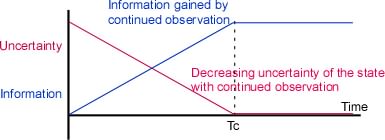
If X is a discrete system, there is a limit to how much
information can be gained about X by observing it. If the
global uncertainty of X (what you believe about X before
observing it) is U(X), no amount of observation can reduce
that uncertainty below zero – the value of U(X) when you
know the state of X exactly. Accordingly, the information
gained by continued observation of a static quantity
plateaus at the global uncertainty of that variable – the
amount that the observer did not know about it before
starting the series of observations.
        (Figure 1)

        This is one place where the difference between continuous
and discrete variables matters. If the system X has a finite
number, N, of distinguishable states, its uncertainty cannot
be greater than log(N), so log(N) is the maximum amount of
information that could be obtained about it by continued or
repeated observation. But if the states of X form a
continuum, it has an infinite number of states, meaning that
in theory there is no limit to the amount of information
about it that could be gained by continued observation. In
practice, of course, the resolution of the observing system
imposes a limit. Precision is never infinite, even if the
limit is imposed by quantum uncertainty.
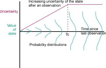
What about the situation in which X is or may be changing?
If a changing X is observed once, the uncertainty about X
becomes a function of time since the observation. X may
change state continuously or abruptly, slowly or fast.
However it may change, the “information rate” of X is
defined as dU(X)/dt provided that the observation timing is
independent of anything related to a particular state or
state change of X.
        -----------

        [Aside: Here we have another example of the kind of
complementarity between two measures that is at the heart of
the Heisenberg Uncertainty Principle of quantum mechanics.
If you know exactly where something is, you know nothing
about its velocity, and vice versa. The rate at which you
get information from observing something can tell you about
both its value and the rate of change of value, but the more
closely define one of these, the less you can know about the
other. The information rate determines the size of the
“precision*velocity” cell.]
        -----------

        If an observation is made at time t0 and never thereafter,
immediately after the observation at time t0+e (“e”
represents “epsilon”, a vanishingly small quantity) the
uncertainty of X is U_(t0+e)(X) . From that moment, U_t(X)
increases over time. The rate at which U_t(X) increases
depends, in the casual tautological sense, on how fast the
value of X changes. If the variable is a waveform of
bandwidth W, this can be made a bit more precise. The actual
rate depends on the spectrum of the waveform, but for a
white noise (the worst case) the rate dU/dt =
Wlog(2pieN) where N is the noise power (which again
depends on the choice of units).
However, just as continued observation cannot yield more
information than the initial uncertainty of X, so continued
external influences or other cause of variation cannot
increase U_t(X) beyond its global value (its value
determined from the long-term statistics of X).
        (Figure 2)

        ----------

        3. Information and history

        In this section, we are interested in the mutual information
between the preceding history and the following observation,
which is symbolized M(X|Xhistory). In everyday language, we
want to know how much we can and cannot know about what we
will observe from what we have observed.
Mutual information need not be just between the states of
system X and the states of a different system Y. It can be
between the states of system X at two different times, which
we can call t0 and t1. If t0 and t1 are well separated, the
state of X at time t0 tells you nothing about its state at
time t1. This would be the case at any time after Tc in
Figure 2. But if t1 follows t0 very closely (i.e. near the
left axis in Figure 2), it is very probable that the state
of X has not changed very much, meaning that the Mutual
Information between the two states is large. They are highly
redundant, which is another way of saying that the mutual
information between two things is close to its maximum
possible value.
Suppose X is the weather. If it is sunny at 10 o'clock, it
is likely to be sunny at one second past ten, or one minute
past ten. The probability of it remaining sunny is still
pretty high at 11, and still moderately high at ten
tomorrow. But by this time next week, the observation that
it is sunny now will not tell you very much more about
whether it will be sunny then than will a book about the
local climate at this time of year.
As the example suggests, M(X_t:X_(t-tau)) -- the complement
of U_(t-tau)(X|observation at t0) shown in Figure 2-- is a
function of tau that usually decreases with increasing tau.
I say “usually”, because it is not true of periodic or
nearly periodic systems. The temperature today is likely to
be nearer the temperature this time last year than to the
temperature at some randomly chosen date through the year.
For now we will ignore such cyclic variation, and treat
M(X_t:X_(t-tau)) as if it declined with increasing tau,
until, at some value of tau, it reaches zero.
        ------footnote-------

        For a signal of bandwidth W, M(X_t:X_(t-tau)) reaches zero
at tau = 1/2W. No physical signal is absolutely restricted
to a precisely defined bandwidth, but the approximation can
be pretty close in some cases. Good audio sampling is much
faster than 1/2W because the physical signals of musical
instruments have appreciable power at frequencies well about
the listener’s hearing bandwidth.
-----end footnote-----
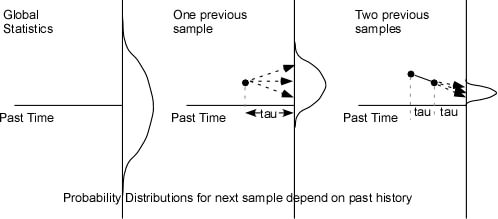
Suppose a signal is sampled at regular intervals separated
by tau seconds, with tau small enough that knowledge of the
signal value at one sample reduces the uncertainty of the
state of the next and previous samples. The probability
distribution of the next sample is constrained by the values
of the previous samples. One might think of the value of the
sample as being that of a perception, but that is not
necessary.
        (Figure 2)

        Figure 2 suggests how knowledge of the past values may
constrain the probability distribution of the next sample
value when the inter-sample time, tau, is short compared to
the rate of change of the variable.
The first panel suggests the uncertainty of the next sample
if one knows nothing of the history of the variable. If the
variable is from the set of possible states of X, its
uncertainty is U(X). The second and third panels show how
the uncertainty is reduced if the values of the previous one
or two samples are known. In the middle panel, one possible
value of the previous sample is shown, and in the third
panel the values of the two previous samples are taken into
account.
The figure is drawn to show the changes in a slowly changing
waveform, but that is just one possibility. It could equally
easily represent the probabilities in a sequence of letters
in a text. For example, the left panel might represent the
possibility of observing any letter of the alphabet, the
middle the distribution of the next character after
observing a “t”, and the right panel the distribution of the
following character after observing “th”. Since we assume
that the statistics of X are stationary (i.e. do not depend
on when you sample them, provided that choice of the
sampling moment is independent of anything happening in X),
M(X0:X1) = M(X1:X2) = M(X2:X3)…
We want to know the uncertainty of X at a given moment t0
given its entire previous history. If X is a slowly varying
waveform, its uncertainty knowing the previous history right
up to t0 is zero, which is uninteresting. In that case we
have to ask about its history only up to some time t0-tau.
We will actually consider the history to consist of
successive samples separated by tau seconds. In the case of
a discrete system such as the letters of a text, no such
restriction is required, but by making the restriction on
the sampling of the continuous waveform we can treat both
kinds of system similarly.
        Formally, one can write

        U(X0|History) = U(X0) - M(X0:History)

        but that is not much use unless one can calculate the mutual
information between the next sample value x0 and the history
of system X. It is possible again to write a general
formula, but its actual calculation depends on the
sequential statistics of X.
The History of X can be written as a sequence of samples
counting back from the present: X1, X2, X3, … and
M(X0:History) can be written M(X0:X1, X2, X3,…)
M(X0:History) = M(X0|X1) + M(X0:X2|X1) + M(X0:X3|X2,X1) +
M(X0:X4|X1,X2,X3) + …
In words, the mutual information between the next sample and
the history can be partitioned into the sum of an infinite
series of mutual information elements, each one being the
amount one sample contributes to the total mutual
information, given the specific values of all the samples
between it and the most recent sample.
To make this concrete, let's consider a few specific
examples
        --------

        Example 1: X is a sequence of symbols "a" and "b", that
alternate “…ababab…”
If one looks at an arbitrary moment, one has an 0.5 chance
of the next sample being a or b: U(X0) = 1 bit. If one has
seen one sample, which might have been either a or b, there
is no uncertainty about the next sample: U(X0|X1) = 0, which
gives M(X0:X1) = U(X).
What then of M(X0:X2|X1)? Remember that M(A:B) cannot exceed
the lesser of U(A) and U(B). In this case, U(X2|X1) = 0
because if X1 was a X2 must have been b, and vice-versa. So
M(X0:X2|X1) = 0 and all subsequent members of the series are
also zero.
One can extend this example to any series or waveform that
is known to be strictly periodic with a known period.
        -------

        Example 2: X is a sequence of symbols a, b, and c with the
property that a is followed equally probably by b or c, b by
c or a, and c by a or b. No symbol is ever repeated
immediately, but apart from that, each other symbol is
equally likely at any sample moment.
        U(X0) = log(3) = 1.58 bits

        U(X0|X1) = 1 bit, which gives

        M(X0:X1) = 0.58 bits

        It is irrelevant how X1 took on its value from X2. If x1 =
a, x2 could have equally well been b or c. Therefore
        M(X0:X2|X1) = 0

        --------

        Example 3. X is a sequence of five different symbols
labelled 1, 2, 3, 4, 5. Considering 5 and 1 to be
neighbours, each symbol can be followed by itself with
probability 0.5 or one of its neighbours with probabiity
0.25. Over the long term, each symbol appears with equal
probability.
        U(X0) = log(5) = 2.32 bits

        U(X0|X1) =-0.5 log 0.5 - 2* (0.25 log 0.25) (because the
probability is 0.5 its predecessor was itself and 0.25 that
it was either of its two neighbours)
                       = 0.5 + 0.5 = 1 bit

        M(X0:X1) = 2.32 - 1 = 1.32 bits

        M(X0:X2|X1) depends on the relationship between X2 and X0,
unlike the situation in example 2. There are five
possibilities for x0 (the value of X0). the probability of
these five depends on the relationship between x0 and x2. We
must consider each of these five, and partition M(X0:X1)
according to the probabilities for each value of X2. In a
formula:
        M(X0:X2|X1) = Sum_k(p(X2=xk)*M(X0:X2|X1=xk))

        Since the probability p(X2=xk) is the same for each value of
xk (all symbols are equally likely over the long term), this
sum comes down to
        M(X0:X2|X1) = (1/N)*Sum_k(M(X0:X2|X1=xk))

        We consider all these possibilities individually. Since all
the relationships are symmetric (meaning that it doesn’t
matter which value we select as the possible next sample,
x0), we need deal only with the relationships themselves.
The sequence could be {x0, x0, x0}, {x0, neighbour, x0},
{x0, neighbout, neighbour} or {x0, neighbour,
non-neighbour}. Examples of each might be {3.3.3}, {3,4,3},
{3,4,4} and {3,4,5}, which would have probabilities 0.50.5
= 0.25, 20.250.25=0.125, 20.250.5=0,25, and
0.250.25=0.125 respectively.
There is no need to do the actual calculations here. They
are easy but time-consuming. The point is that we can
calculate M(X0:X2), M(X0:X2|X1) and the rest directly from
the conditional probabilities.
        ---------

        Example 4: X is built by summing a succession of samples of
another system Y, such that xj = Sum(History(X)) + yj, x0 =
0 for some specified value of k, and yj is a sequence of
positive and negative integer values, samples from a system
Y, that average zero. In this example, the numbering scheme
goes in the direction of time, later samples being labelled
with larger numbers. At the k’th sample the expression
M(X|Xhistory) becomes
        M(Xk:Yk|X_(k-1), X_(k-2), ... X(0))

        Each sample of Y contributes equally to the value of X, so
there is no need to consider the sequential order of the y
values. Assuming that Y is a series of numerical values and
the samples of Y are independent, the variance of X
increases linearly with the number of samples, so its
standard deviation increases proportionally to the square
root of that number.
Let us trace the contribution of the first few samples of Y
to the uncertainty of X.
After one sample, y0, of Y, x0 will equal y0, which means
U(X0) = U(Y0).
        M(X0:Y0) = U(X) + U(Y) - U(X,Y) = U(X) = U(Y)

        After the next sample, U(X1) still is given by the formula
Sum(p log p), but the probabilities are no longer the same
as they were before the first sample. There is a wider range
of possibilities, from twice the minimum value of Y to twice
the maximum value of Y, and the probabilities of those
possibilities are not equal. Because the probability
distribution over the possible values of X is not uniform,
U(X) < 2*U(Y).
As more and more samples are included in the Sum, the range
of X increases, but values near zero come to have higher and
higher relative probabilities. The distribution of
probabilities over the possible values of X approaches a
Gaussian with variance that increases linearly with k, so
U(X) approaches U(Y)sqrt(k). The ratio U(X)/(kU(Y)
decreases with increasing k, approaching 1/sqrt(k) as k
becomes large .
We want to consider the contribution of the k'th sample of
Y. How much does the kth sample of Y reduce the uncertainty
of the k+1th value of the Sum, as compared to knowing only
the History up to the previous sample? That is the mutual
information between the kth sample of Y and the k+1th value
of X.
For large k, (U(X_k) - U(X_(k-1)))/U(Y) approaches
sqrt(k)-sqrt(k-1), an increasingly small number. Yet it
remains true that U(X_k|History) - U(X_k|History, Yk) =
U(Y). The uncertainty of the value of X after the next
sample of Y is always the uncertainty of Y, because if you
know the current value of X, the next value is determined by
the value of the Y sample. How can these two statements be
reconciled? The key is the conditional of knowing the
History. Without the prior History (in this case the Sum),
the contribution of each successive Y sample to the
uncertainty of X becomes less and less, but if you do have
the prior History, the value of the next X sample will have
an uncertainty that is the uncertainty of the Y sample.
The situation is the same if the system X is normalized,
meaning that its variance is independent of the number of
prior samples after a sufficient number of Y values have
occurred. The magnitude of the contribution of the k’th Y
sample is reduced proportionally to sqrt(k), but its
contribution to the various uncertainties are the same,
provided that the different possible values of X are
resolved.
        --------

        Example 5: The same as Example 4 except that the samples of
Y are not independent. If Y is a continuous waveform, the
samples are taken more closely than the Nyquist limit
(samples separated by 1/2W, where W is the bandwidth of the
waveform). If Y is a discrete set of possibilities,
successive samples are related by some kind of grammar. The
two kinds of possibility converge when the discrete set of
possibilities is linearly arranged and the grammar merely
makes transitions among nearby values more likely than
across distant values.
The new issue here is that if the history of Y is known,
U(Yk) < U(Y). Therefore M(Xk:History(X), yk) < U(Y).
Each successive sample of Y reduces the uncertainty of X
less than would be the case if the samples of Y were
independent of each other. The difference is subsumed by the
fact that M(Xk|History(X)) is greater than it is in the case
when the Y samples are independent, by the same amount.
        ---------

        Example 6: System X is a function of the current and past
samples of system Y. We want to know the uncertainty of
sample xk when the values of successive Y samples are known
only up to sample y_(k-h). For example, in the grammar of
example 3, we may have observed the sequence 1,2,1,5,
(samples y1, y2, y3, y4) and want to know the uncertainty of
sample x6, which is a function of y1, y2, y3, y4, y5, and
y6. We do not yet know the values of y5 or y6. As a
real-world example, a trader in the days of sailing ships
might have known the market conditions in China and England
several months before his ship captain actually bargains for
tea in Canton, but the earlier conditions are the conditions
on which he must base his instructions to the captain.
==========End=========