···
On Mon, Jul 18, 2016 at 5:12 PM, Alex Gomez-Marin agomezmarin@gmail.com wrote:
Â
AGM: First, Rick, your demo hardly proves anything because you inject ad hoc temporal dynamics in the references whose lawful (or unlawful) properties will simply be reflected by the control system, which does hardly more than integrating them.Â
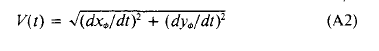
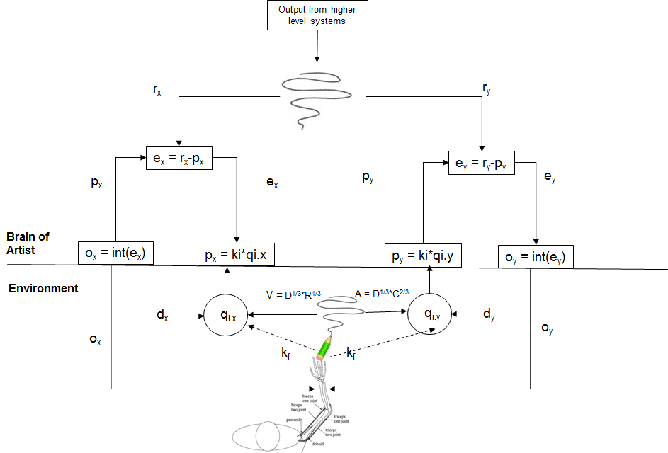
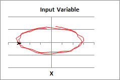
RM: OK, let’s start from the beginning. The goal of this exercise is to develop a model that explains how people (and other organisms) produce curved paths that have the property that the velocity of movement while producing the path (V) is proportional (by a power function) to the curvature of the path at each instant. So my first step was to develop a control model of someone like an artist drawing a curved line. The model is diagrammed below:
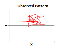
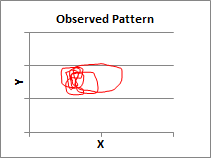
RM: The phenomenon to be accounted for by the model is the curved pattern (squiggle) produced by the artist. The completed squiggle is shown at the bottom of the figure, in the environment where the squiggle is actually produced. The model has to produce this squiggle exactly as the artist produced it, by varying the position of the pen over time. According to PCT, the observed variations in pen position (qi.x and qi.y) are controlled results of variations in the reference specifications (r.x and r.y) for the perception of those positions (p.x and p.y). Therefore the model varies these references in a way that would produce the observed variations in qi.x and qi.y.Â
RM: r.x and r.y are the references that you object to, claiming that they contain ad hoc temporal dynamics. I question whether they do, but I agree that it looks trivial (and a lot like cheating) to put the desired end result (the squiggly movements of the qi.x and qi.y over time) into the model (in the form of the identical squiggly movements of r.x and r.y). But that is the way the PCT model works; controlled (intended) results are results that match specifications set autonomously by the organism itself.Â
RM: But the reference signals in the control model are not “cheating” any more than are the  “command” signals in motor control models of behavior, like that of Gribble/Ostry, which is shown below. The commands in the model are commands for output; forces that will produce movements of the pen that will result in the observed squiggle. In the PCT model, references, r.x and r.y, are commands for input; perception that match the reference specifications.
RM:Â So both models have to use internal commands in order to produce the observed result (squiggle). The difference is that the commands in the PCT model “look like” the observed result; the commands in the Gribble/Ostry don’t necessarily “look like” the result produced. But in both cases the commands have to be carefully crafted to produce the correct result. So the possibility of introducing “ad hoc temporal dynamics” is present in both models. But the PCT model can do something that the Gribble/Ostry cannot do: it can control. That is, it can produce the intended squiggle in the face of disturbances.Â
RM: Although the variations in the references (r.x, Â r.y) in the PCT model correspond to the squiggle that is produced (qi.x, qi.y) , I didn’t expect this simple model to produce a squiggle with a power function relationship between angular velocity (V) and curvature (R). I assumed, like you, that the power law relationship was either 1) a controlled result in itself (the person controlling for speeding up through tighter turns), which would require a whole extra control organization in the model or 2) the result of complex dynamic characteristics of muscle force production (the functions of e.x and e.y in the control model diagram above) and/or of the feedback function connecting force output to pen movement input (k.f in that diagram).Â
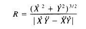
RM: So I was very surprised to find that the squiggle produced by this simple control model showed a power relationship between V and R . And when the squiggle was an ellipse the coefficient of the power function was about the same (~.31) as that found by Gribble/Ostry for their ellipse production model  – a model with a far more dynamically complex method of generating the ellipse than my control model. That’s when I realized that the observed relationship between V and R might be a mathematical property of all curved lines. And, indeed, it turns out that it is. The relationship between V and R, which can be found using kindergarten math, isÂ
V = Â |dXd2Y-d2XdY|Â 1/3Â *R1/3Â Â Â
RM:  Note that the term  |dXd2Y-d2XdY|, which I called D, implying that it was a constant, is a variable. So the value of V for any curve is proportional (exactly) to the 1/3 power of |dXd2Y-d2XdY| and the 1/3 power of R.  I was as surprised by this as as anyone. So I wanted to make sure it was true so I did the multiple regression analysis using log ( |dXd2Y-d2XdY| ) and log (R) as predictors of log (V) for many different “squiggles” and always found that all the variance in log (V) was accounted for by an equation of the form:
log (V) = .33* log (|dXd2Y-d2XdY|) +.33* log(R)Â
AGM: Second, you are stubbornly confused about the difference between a mathematical relation (that allows to re-express curvature as a function of speed, plus another non-constant term that you insist in ignoring and treating like a constant),
RM: I hope you see now that I do not treat the variable  |dXd2Y-d2XdY|  as a constant. The mathematical relationship is as flawless as my kindergarten math teacher;)
Â
between a physical realization (the fact that one can in principle draw the same curved line at infinitely different speeds),
RM: Actually, I understand that the same curved line (squiggle) can be produced at an infinity of different speeds and by an infinity of different means (different variations in o.x and o.y producing the same squiggle, qi.x, qi.y). The same relationship between V and R holds regardless of the speed with which the squiggle is produced and and the means used to produce it. The relationship between V and R is always:Â
log (V) = .33* log (|dXd2Y-d2XdY|) +.33* log(R)Â
RM: This same relationship between V and R even holds for all the different squiggly patterns made by o.x and o.y to  produce the same squiggly pattern --qi.x, qi.y.Â
AGM: and between a biological fact (that out of all possible combinations of speed and curvature, living beings are, for yet some unknown reason —but there are tens if not hundreds of papers making proposalsâ— constrained following the power law,
RM: But now we know the reason. It’s a result of the fact that the relationship between V and R for any curved line is
V = Â |dXd2Y-d2XdY|Â 1/3Â *R1/3Â Â Â
RM: There is no way to draw a curved line so that this equation does not hold. So there is no biological constraint that creates the observed power law; it’s a mathematical constraint.Â
RM: The reason people have found different power coefficients for the relationship between V and R is because they have left the variable  |dXd2Y-d2XdY|  out of the analysis. When you leave  |dXd2Y-d2XdY|  out of the analysis, variations in that variable can lead to different estimates of the power coefficient of R. The amount by which the value of the power coefficient of R is affected by leaving  |dXd2Y-d2XdY|  out of the analysis depends on the shape of the squiggle that is drawn. Leaving  |dXd2Y-d2XdY| out of the analysis of the V/R relationship for an ellipse affects the actual power coefficient of R (.33) very little, so the value obtained is around .31 (see Gribble and Ostry, Table 1). Other squiggles can bring the power coefficient of R down as low as .2.Â
RM: On that note, Martin Taylor noted that the power coefficient for R, which is around .33 for a curved figure drawn in the air, is closer to .25 when the same figure is drawn  in a viscous medium (like water). It turns out that this can be explained in terms of a difference in the feedback function (k.f in the diagram) in the two cases.Â
RM: In the PCT model, the feedback function is a simple, linear coefficient. When the model traces out an ellipse with a feedback function of k.f = 1.0, the power coefficient of R is .32; when the feedback function is changed to k.f = .5 – equivalent to trying to move a pen through a more resistive medium – the power coefficient of R is .26. This happens simply because the ellipse drawn in the resistive medium is a little sloppier than the one drawn in the air. The change in feedback function changes the loop gain of the control system.Â
AGM: But you will now reply for the n-th time saying that everybody that has ever worked on the power-law misses the point of control systems and that your toy demo proves they don’t get it.
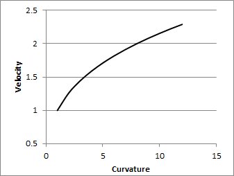
RM: Yes. But they have been fooled by a rather convincing illusion. It’s hard not to see the observed relationship between V and R as a situation where the agent purposefully changes speed through curves (the power law actually suggests that agents increase their speed as the curve increases, but this increase in speed decreases as curvature increases; it does not suggest that control systems tend to slow down around sharp curves).
RM: So I agree that it is very surprising (and, perhaps, disappointing) that the relationship between V and R tells us nothing about how people draw curves. But that doesn’t mean that research on how people (and other organisms) produce curved paths should come to an end. To the contrary, it opens up new and fruitful questions about exactly how this is done. For example, the integral output function that I use in the existing model is obviously an over simplification. Something like the  Gribble/Ostry model pictured above is probably a closed approximation. A clever experimenter should be able to design behavioral (and/or physiological) studies to determine what the best model of the output function is.Â
RM: Going “up a level” (so to speak) research could also be aimed at determining how what are presumably higher level control systems set the references for the x,y coordinates of the figure being drawn (assuming that the figure is a controlled result and not a side effect of controlling other variables, as in the CROWD demo).Â
RM: So there is really a lot of very important and challenging research to be done in order to understand how people draw figures. But this research must be based on an understanding of the fact that the figure drawn is a controlled variable – an intended result. And so any research aimed at understanding how figures are drawn must be based on an understanding of how control works.Â
AGM: But, again, you gloss over serious flaws interpreting the difference between mathematical equations, physical conditions and biological constraints as facts, and you magnify the relevance of a toy demos that, I wish could shed new light, but so far don’t shed much new to the problem.
RM: I hope this post helps. I don’t believe I have glossed over flaws. But if there are substantive flaws please point them out. As I said above, if my analysis is correct that doesn’t mean all is lost. Indeed, I think it actually opens up many new and very productive possibilities for research.Â
Best regards
Rick
So I encourage you (and everyone still reading these email exchanges) to say something new and relevant, because I still believe that asking what is being perceived and what is being controlled is worth-while in figuring out why speed and curvature are constrained they way they are.
Â
Alex
–
Richard S. MarkenÂ
“The childhood of the human race is far from over. We
have a long way to go before most people will understand that what they do for
others is just as important to their well-being as what they do for
themselves.” – William T. Powers