···
[From Rick Marken (2016.07.16.1415)]
There is a considerable body of research aimed at understanding the power law relationship between curvature and angular velocity that is observed when people (or other organisms) move (or move things , like pens) along curved trajectories. The power law can be expressed as follows:
V = K*Rb (1)
where V is angular velocity, defined as
V = (X2*Y2 )1/2 (2)
and R is curvature, defied as
R = [(X2Y2 )3/2]/|dXd2Y-d2X*dY| (3)
What equation (1) says is that when you are drawing a figure, such as an ellipse, for example, the speed of your movement at each instant (V) is proportional to the degree of curvature at that point ®; that is, you move faster through steep than shallow curves. According to Gribble and Ostry (Journal of Neurophysiology, v. 76, 1996) the value of the power coefficient, b, estimated under a “variety of experimental conditions” has been consistently found to be about 1/3.
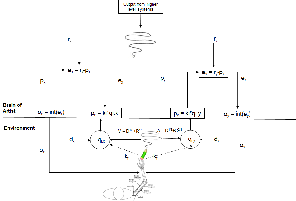
Researchers have tried to explain the observed power relationship between V and R. These explanations have taken the form of open-loop, output generation models, such as the one described in Gribble and Ostry (1996, Fig. 1). The Gribble/Ostry model assumes that hand drawn figures, like ellipses, are the result of motor programs that send the appropriate signals to the muscles to generate the forces that move the hand in a elliptical pattern in such a way that there is a power relationship between the speed with which the hand moves and the curvature of the figure being drawn (an ellipse in this case). The Gribble/Ostry model successfully generates ellipses like those drawn by people and these ellipses show the power law relationship between V and R with a b coefficient of about 1/3. And, like people, the coefficient of the power law relationship remains about 1/3 whether the ellipse is drawn rapidly or slowly.
I developed a closed loop control model of ellipse drawing. It was an extremely simple model in the sense that there were no complex output calculations. The model simply produced outputs that kept a perception of the state of an input variable (qi.x, qi.y) matching elliptically varying references (r.x, r.y). When I computed the relationship between V and R for the ellipses drawn by the model I found that there was a perfect power relationship between V and R with a b coefficient value of exactly 1/3 (.33). This was a very puzzling result; here I was getting a very nice power relationship between V and R, just like what had been observed empirically and what had resulted from the output generation model of Gribble and Ostry, and I was getting it from what seemed like a trivially simple model. T**hen it struck me that this must mean that the observed power relationship between V and R could not possibly be a result of the way the ellipse was generated; it had to be a property of the ellipse itself. Which led me to take another look at the equations for V and R (equations 2 and 3 above). And I realized that it would be possible to combine the two equations and solve for V as a function of R. The result was:
V = K*R1/3 (4)
where K = |dXd2Y-d2XdY| . This is the power law relationship that has been observed to exist between V and R and the coefficient is 1/3, the same as the value of b which, according to Gribble and Ostry, is estimated under a “variety of experimental conditions”. So the relationship between V and R that is observed in movement studies simply reflects a mathematical relationship between these variables; it has nothing to do with how the movements are produced!!
The mathematical power relationship between angular velocity and curvature exists even if these variables are measured as angular velocity = A=V/R and curvature = C=1/R. The observed relationship between A and C is again a power relationship of the form:
A = K*Cb (5)
with b typically found to be approximately 2/3 rather than 1/3 as it is in the relationship between V and R. When you do the algebra that converts equation (4) into a form involving A and C you get the following:
A = K*C2/3 (6)
where K = D1/3 . Again, there is a power relationship between A and C as there is between V and R and the coefficient of this mathematical relationship is close to the empirically observed coefficient, 2/3.
This is a startling result. It means that students of the power law of movement control have been mistaking a mathematical fact for empirical evidence regarding how movement is produced. It is like doing research on how people draw circles and taking the observation that the circumference of the circles they draw are always close to being equal to p times the diameter as a fact that says something about how the circles are drawn.
So how could researchers in this area have missed the fact that there is a mathematical power relationship between V and R (with a power of 1/3) and between A and C (with a power of 2/3)? It can’t be because these researchers were not as good at math as I am; the papers I’ve been reading are bristling with high powered math and I had to get help from my math teacher son to derive equations 4 and 6. No, I think the reason I discovered this alarming fact and others didn’t is because the latter were looking at the behavior under study (drawing figures) through causal theory glasses while I was looking at the behavior through control theory glasses.
Through causal theory glasses, drawing an ellipse (for example) looks like a caused output – the result of precisely calibrated neural signals sent to the muscles; these signals are thought to create just the right forces over time so that the resulting hand movement is an ellipse. The observed power relationship between angular velocity and curvature is then taken as evidence of how the nervous system generates the neural signals that produce the ellipse; it generates signals so as to maintain a power relationship between speed of movement and the size of the curve through which the movement is being made.
But through control theory glasses, drawing an ellipse looks like a controlled (rather than a caused) result of muscle forces – a controlled variable. This means that the same result – an ellipse – cannot be consistently produced by the same neural signals (and resulting muscle forces), even if those signals are precisely calibrated. That is because the same neural signals will have different effects on the controlled result under difference circumstances. The different circumstances are the changing fatigue levels of the muscles that produce the result (ellipse), the changing conditions of the surface on which the ellipse is drawn, and so forth. These changing circumstances can be lumped together in my model of ellipse production as varying disturbances to the state of the controlled variable – the elliptical movement of the pen in the X and Y dimension, qi.x, qi.y.
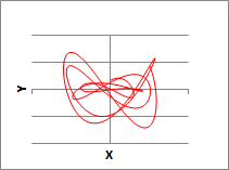
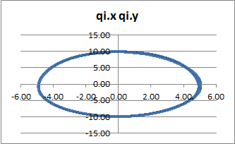
The results of a simulation run with moderate level disturbances are should in the graphs below. The top graph shows the ellipse drawn by the two control systems, one controlling pen position in the X dimension (qi.x) and the other controlling pen position in the Y dimension (qi.y). The ellipse traced out is almost exactly the same as the ellipse specified by the time varying values of the reference signals, r.x and r.y, that are sent to the systems controlling qi.x and qi.y, respectively. This looked like a pretty trivial result when the ellipse was produced in a disturbance free environment. But in this case there were moderately intense disturbances present. So the outputs that produced this result were not elliptical, as can be seen in the next graph.
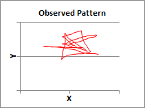
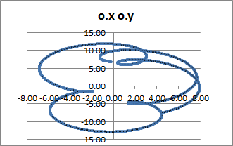
The graph below shows the output variations that produced the elliptical result above. The outputs are clearly not elliptical; they had to vary as necessary in order to compensate for disturbances that would have prevented production of the ellipse.
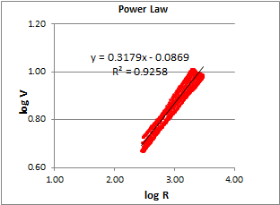
The chart below shows a plot of log V versus log R for the elliptical figure above (plot of pen movement; qi.x, qi.y). If there is a power law relationship between V and R it will show up as a good linear fit on a log-log plot. And indeed, there is an excellent linear fit (R2=.92) with a coefficient, corresponding to b of .32, almost exactly .33. This power law relationship was produced by outputs that result in a power law but one that is quite different than that for the ellipse.
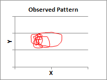
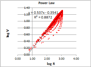
The graph below shows the power law relationship between V and R for the output trace (o.x, o.y) that produced the ellipse (qi.x, qi.y). The fit to a power law is not as good for the outputs (o.x,o.y) as for the result of the controlled variable(qi.x,qi,y) but it is still a pretty good fit (R2 = .88). But the coefficient of the power relationship is not nearly as close to 1/3 as it was in the case of the ellipse. I believe this is because odd shaped curves, like those of the o.x,o.y) can result in variations in K that obscure the 1/3 power component of the relationship between V and R. The variations in K result from variations in dX, dY,d2X and d2Y since K = |dXd2Y-d2XdY|.
I think the most important lesson here is that you have to understand that behavior is a control process before you can start doing research to determine how this behavior is carried out. The problem with the velocity-curvature power law research is not that the researchers are using the wrong theory (although they are); the problem is that they are looking at the wrong phenomenon. They think they are studying caused output when, in fact, they are studying controlled input. You have to get the phenomenon right before you can get the theory right. In the case of the power law, the bias to see behavior as caused output seems to have blinded the researchers to the fact that they are seeing a mathematical law of curved lines rather than the psychophysiological law of movement that they think they were seeing. This is another version of what Powers called “The Behavioral Illusion” – the illusion of seeing causality where, in fact, there is control.
Best
Rick
–
Richard S. Marken
“The childhood of the human race is far from over. We
have a long way to go before most people will understand that what they do for
others is just as important to their well-being as what they do for
themselves.” – William T. Powers