RM: No, that is not my “theory”. Something can be a real phenomenon and a statistical artifact.
No, it cannot. Name some other examples that are real phenomena and also statistical artifacts.
RM: But what is seen is a statistical artifact that results from the failure to include the variable D in the regression.
Well, that is your theory then. You prefer to call it a hypothesis? The speed-curvature power law is a statistical artifact that results from the failure to include the variable D in the regression.
Are you saying it is not possible to test weather something is a statistical artifact, but it just has to be because of the algebra?
I’ll just back up a second to establish the terms.
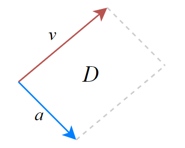
v is the velocity vector, with components x’ and y’
a is the acceleration vector with components x’’ and y’’
D is the area closed by a and v, calculated as the magnitude of the cross product of a and v, as in (1), or by components of a and v, as in (2)
(1) D = | a x v |
(2) D = | y’‘x’ - x’‘y’ |
You are saying that the area D closed by vectors a and v, should be included in the regression analysis between V (speed, magnitude of v, one side of the parallelogram) and C, even though D is directly determined by V?
If a is has constant magnitude, the blue side of the parallelogram is always the same. All of the variance in D is going to come from variance in V. Agreed?