[Rick Marken 2018-08-26_15:19:21]
RM:… The “noise” added by Maoz et al simply produces a different trajectory but one where the correlation between curvature and affine velocity is still relatively low so that the “power coefficient” in an omitted variable regression (one that leaves out affine velocity) is still close to the power law value (-1/3 in their case).Â
AM:Â The noise produces a “jittery” trajectory, as you can see in their illustration. If it there is any correlation, it is an artifact of the noise.
 RM: There is some degree of correlation between curvature and affine velocity in all movement trajectories. This correlation varied somewhat over the normally distributed samples trajectories analyzed by Moaz et al. but was surprisingly consistent. When they added noise to non-power law trajectories – trajectories with power coefficients that were essentially zero rather than -1/3 – they found that you would get power law conforming trajectories – trajectories with power coefficients that are close to -1/3 – with very little added noise. This means that with very little noise added to a trajectory you can change the correlation between curvature and affine velocity from 1.0, which results in a power coefficient of 0, to 0.0, which results in a power coefficient of -1/3. These variations in the observed power coefficient are due only to variations in mathematical characteristics of the movement trajectories themselves. The characteristic of a trajectory that makes the difference in terms of whether or not it conforms to the power law is the correlation between curvature and affine velocity.Â
AM: And they are not doing omitted variable regression
RM: Actually, they did. Whenever you regress curvature on velocity, omitting affine velocity as a predictor, you are doing an omitted variable regression. In other words, power law researchers always do omitted variable regression to see if a trajectory conforms to the power law.Â
RM: What is more important is that Moaz et al did an omitted variable bias (OVB) analysis, just as we did (Marken and Shaffer, 2017). Their analysis, like ours, showed that a regression analysis that includes only curvature as a predictor of velocity, omitting affine velocity as a predictor, will find a power coefficient that deviates from the power law coefficient (-1/3, 1/3 or 2/3, depending on how curvature and velocity are measured) by an amount proportional to the correlation between curvature and affine velocity.Â
RM: The Moaz et al OVB analysis is given in their equation (6):
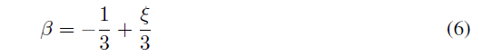
RM: This is equivalent to equation (12) in Marken and Shaffer (2017):

RM: The d (delta) in our equation (12) is equivalent to x/3 (x/3) in their equation (6), where x (x) is equal toÂ
Covariance [log(curvature), log(affine velocity)]/ Variance [log (curvature)]
RM: b’obs (beta’.obs) in our equation (12) is equivalent to b (beta) in their equation (6). We call ours  b’obs (beta’.obs) because it is the power coefficient -- b (beta) – that is observed when one does a regression of curvature on velocity while omitting affine velocity, which is the variable we called D and that they call a (alpha). Finally, btrue (beta.true) in our equation (12) is equivalent to -1/3 in their equation (6). We called it btrue (beta.true) because it is the coefficient of curvature in the formula that gives the linear relationship between curvature and velocity. For Marken & Shaffer (2017) this formula was:Â
log (V) =1/3log (R)Â +1/3 log(D)Â
and for Moaz et al (using equivalent names for the variables) it was
log (V) = -1/3log (1/R)Â +1/3 log(D)Â Â Â
RM: So in our OVB analysis, btrue (beta.true) is 1/3 and in the Moaz et al OVB analysis btrue (beta.true) is -1/3.Â
RM: So Moaz et al found exactly what we found: When affine velocity is left out of the regression analysis that is used to determine whether or not a movement conforms to the power law, the power coefficient relating curvature to velocity that is found by this omitted variable regression will deviate from the power law value – the mathematically “true” value of -1/3, 1/3 or 2/3, depending on how velocity and curvature are measured – by an amount proportional to the covariance between curvature and affine velocity (per equation (6) in Moaz et al and equation (12) in Marken and Shaffer (2017).
RM: This is what I mean when I say that whether or not you find that a movement trajectory follows the power law depends on the nature of the trajectory itself and tells you nothing about how that trajectory was produced. Trajectories where the covariance between curvature and affine velocity is close to zero will be found to conform to the power law; trajectories where the covariance between curvature and affine velocity is high will be found to deviate from the power law by an amount proportional to the size of this covariance.
AM: - affine velocity is dependent both on curvature and speed, and is cannot be an independent predictor.
RM: Predictor variables do not have to be independent (uncorrelated with each other) in multiple regression analysis.Indeed, they virtually always dependent on each other to some extent. When you do a multiple regression analysis on movement trajectories using both curvature and affine velocity as predictors of velocity you find that the regression coefficients for these variable are exactly the ones in the mathematical equation relating velocity to curvature. That is, if you use V as the criterion variable, and 1/R and D as the two predictor variables in a multiple regression analysis, then the result will be a regression equation that corresponds exactly to the Moaz et al version of the equation relating curvature (1/R) and affine velocity (D) to velocity:
log (V) = -1/3log (1/R)Â +1/3 log(D)Â Â Â
RM: That is, the regression coefficients will be exactly -1/3 and 1/3 for 1/R and D, respectively, and R^2 will be 1.0.Â
Â
AM: They have one formula like the one in your paper, but a completely different dataset and a completely different interpretation.Â
RM: They got the same results with their dataset as we got with ours. And they gave a completely different interpretation of their results than we did because people don’t like finding out that they have been making a huge mistake in their research. This aversion to believing one is wrong is what kept the US in the war in Vietnam; it’s what keeps Trump supporters Trump, it’s why power law researchers were angry at my PCT interpretation of the power law and it’s why behavioral scientists in general don’t like PCT. And it’s all perfectly understandable in terms of PCT.
RM: That’s fair. I didn’t agree with her interpretation of her math.
AM: Oh, right. Sorry Mr. Fields medalist.Â
RM:Â No need for ad hominum. You’re better than that, Adam.Â
Â
RM: Did you notice the non-power law trajectories in our rebuttal to the reappraisal paper. It turns out that you get both power law and non-power law trajectories produced by both living and non living systems…
 AM: If you look into the literature, you’ll find that no one ever claimed that it is exclusively produced by biological systems…
RM: I would think that that alone would suggest that the power law is not an interesting finding regarding the behavior of organismsÂ
RM: That’s because whether or not a trajectory follows the power law depends on characteristics of the trajectory itself and has nothing to do with how it was produced…
AM: I don’t see any meaning in the first sentence.
RM: What it means is what I showed in the OVB analysis above.Â
Â
RM: So I would say that the correlation between disturbance and output is a side-effect of the existence of a controlled variable; that is, it is a side effect of control. So understanding why we observe a correlation between disturbance and output requires that we know about the existence of a controlled variable. And once we know what the controlled variable is, all possible side effects of controlling this variable can be readily deduced.Â
AM: How about reaction time? The minimum time of reaction is set by the physical limits of the particular control system, like delays, integral lags, etc. That is a side effect of controlling a specific variable, that tells you a lot about a system. Could hint to the level in the hierarchy where the perception is happening, and such interesting things.Â
RM: Good point. If you want to call reaction time a side effect then it can certainly be an informative one. But I’m not sure I would call reaction time a side effect of control in the same way that the disturbance-output relationship is a side effect. Reaction time, in the form of transport lag and output slowing, is an intrinsic component of the control process; you have to put these timing variables into a control model to make it work. But you don’t put the disturbance-output transfer function into a control model to make it work; the relationship between disturbance and output is truly a side effect of the operation of a control system acting to keep a controlled variable in a reference state.
Best regards
Rick
···
On Sat, Aug 25, 2018 at 12:36 PM Adam Matic csgnet@lists.illinois.edu wrote:
It cannot go lower than it does, because of the physical limitations of the system, so you consistently get the same minimum reaction time to the same stimuli. Same with speed and curvature in human movement. They have a consistent relationship under certain experimental conditions.Â
Best,
Adam
–
Richard S. MarkenÂ
"Perfection is achieved not when you have nothing more to add, but when you
have nothing left to take away.�
                --Antoine de Saint-Exupery

