I recently posted the following story to the LessWrong blog. It might be of interest here, although it will be mostly preaching to the converted.
Prof. Sagredo has assigned a problem to his two students Simplicio and Salviati: "X is difficult to measure accurately. Predict it in some other way."
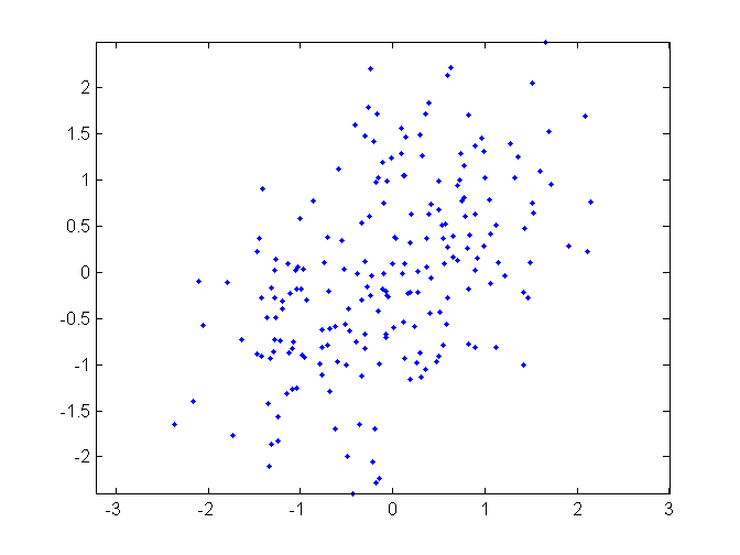
Simplicio collects some experimental data consisting of a great many pairs (X,Y) and with high confidence finds a correlation of 0.6 between X and Y. So given the value y of Y, his best prediction for the value of X is 0.6ya/b, where the standard deviations of X and Y are a and b respectively. A correlation of 0.6 is generally considered pretty high in psychology and social science, especially if it's established with p=0.001 to be above, say, 0.5. So Simplicio is quite pleased with himself.
Salviati instead tries to measure X, and finds a variable Z which is experimentally found to have a good chance of lying close to X. Let us suppose that the standard deviation of Z-X is 10% that of X. A measurement whose range of error is 10% of the range of the thing measured is about as bad as it could be and still be called a measurement. (One might argue that any sort of entanglement whatever is a measurement, but one would be wrong.) It's a rubber tape measure. By that standard, Salviati is doing rather badly.
In effect, Simplicio is trying to predict someone's weight from their height, while Salviati is putting them on a (rather poor) weighing machine (and both, presumably, are putting their subjects on a very expensive and accurate weighing machine to obtain their true weights).
So we are comparing a good correlation with a bad measurement. But how do they compare with each other, rather than with other correlations or other measurements? Let us suppose that the underlying reality is that Y = X + D1 and Z = X + D2, where X, D1, and D2 are normally distributed and uncorrelated (and causally unrelated, which is a stronger condition). I'm choosing the normal distribution because it's easy to calculate exact numbers, but I don't believe the conclusions would be substantially different for other distributions.
For convenience, assume the variables are normalised to all have mean zero, and let X, D1, and D2 have standard deviations 1, d1, and d2 respectively.
Z-X is D2, so d2 = 0.1. The correlation between Z and X is c(X,Z) = cov(X,Z)/(sd(X)sd(Z)) = 1/sqrt(1+d2^2) = 0.995.
The correlation between X and Y is c(X,Y) = 1/sqrt(1+d1^2) = 0.6, so d1 = 1.333.
We immediately see something suspicious here. Even a terrible measurement yields a sky-high correlation. Or put the other way round, if you're bothering to measure correlations, your data are rubbish. Even this "good" correlation gives a signal to noise ratio of less than 1. But let us proceed to calculate the mutual informations. How much do Y and Z tell you about X, separately or together?
For the bivariate normal distribution, the mutual information between variables A and B with correlation c is lg(I), where lg is the binary logarithm and I = sd(A)/sd(A|B). (The denominator here -- the standard deviation of A conditional on the value of B -- happens to be independent of the particular value of B for this distribution.) This works out to 1/sqrt(1-c^2). So the mutual information is -lg(sqrt(1-c^2)).
corr. mut. inf.
Simplicio 0.6 0.3219
Salviati 0.995 3.3291
What can Simplicio do with his one third of a bit? If he tries to predict just the sign of X from the sign of Y, he will be right only 70% of the time (i.e. arccos(-c(X,Y))/pi). Salviati will be right 96.8% of the time. Salviati's estimate will even be in the right decile 89% of the time, while on that task Simplicio can hardly do better than chance. So even a "good" correlation is useless as a measurement.
Simplicio and Salviati show their results to Prof. Sagredo. Simplicio can't figure out how Salviati did so much better without taking measurements on hundreds of samples. Salviati seemed to just think about the problem and come up with a contraption out of nowhere that did the job, without doing a single statistical test. "But at least," says Simplicio, "you can't throw away my 0.3219, it all adds up!" Sagredo points out that it literally does not add up. The information gained about X from Y and Z together is not 0.3219+3.3291 = 3.6510 bits. The correct result is found from the standard deviation of X conditional on both Y and Z, which is sqrt(1/(1 + 1/d1^2 + 1/d2^2)). The information gained is then lg(sqrt(1 + 1/d1^2 + 1/d2^2)) = 0.5*lg(101.5625) = 3.3402. The extra information over knowing just Z is only 0.0040 = 1/250 of a bit, because nearly all of Simplicio's information is already included in Salviati's.
Sagredo tells Simplicio to go away and come up with some real data.
···
--
Richard Kennaway, jrk@cmp.uea.ac.uk, http://www.cmp.uea.ac.uk/~jrk/
School of Computing Sciences,
University of East Anglia, Norwich NR4 7TJ, U.K.