Dead Zones, or Bill was Right (As Usual)

Continuing the discussion from Collective control as a real-world phenomenon:

Eetu said:

This quote from Powers seems really strange for me, especially the last sentence (italics by me):

These two outputs, if about equal, will cancel, leaving essentially no net output to affect the controlled quality. Certainly the net output cannot change as the “controlled” quantity changes in this region between the reference levels, since both outputs remain at maximum.
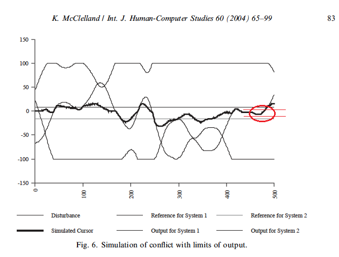
This means there is a range of values over which the controlled quantity cannot be protected against disturbance any more. Any moderate disturbance will change the controlled quantity,…

I think this should mean that if there is an arm wrestling and a tug of war going on between equally strong participants and the situation is frozen so that both participants pull or push with their full strength but the flag or clasped hands don’t move, then in that situation it should be possible for you (if you could do it invisibly) to move the hands or the flag easily back and forth. I really can’t believe this. Has anyone ever tried?

Actually, I did try it last Saturday when I was having dinner with Gary Cziko and his wife. Gary and I arm wrestled while his wife applied gentle disturbances to the position of our clasped hands and they seemed to move easily. So my description, based on Bill Powers’ description, of a Dead Zone that exists when there is a conflict, seems to have been correct. But Kent argues that there is no Dead Zone in his models of conflict. If this were true then Bill’s (and my) description of the Dead Zone was incorrect.

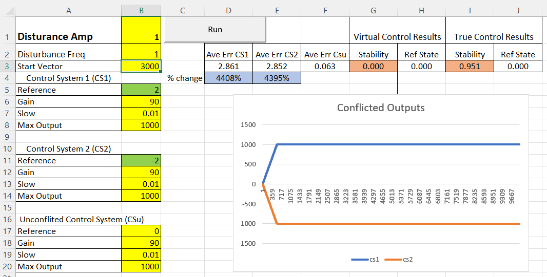
Kent presented the following data as evidence that there is no Dead Zone:

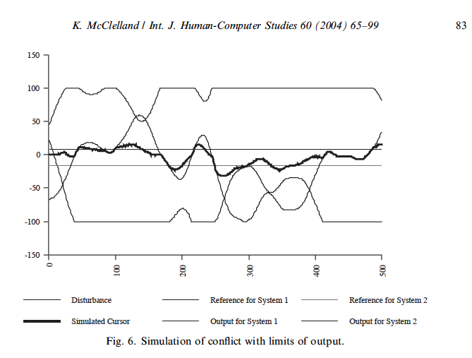
But this is not a proper test for the existence of a Dead Zone. The fact that the conflicted systems correct for disturbance even when limited in the maximum output they can produce does not disprove the existence of a Dead Zone. The Dead Zone is defined as a range of disturbance amplitudes that will not be resisted by control systems in conflict – a virtual control system - but will be resisted by an equivalent unconflicted control system.

I have developed a spreadsheet model that demonstrates the existence of a Dead Zone that exists when two control systems of equal strength – in terms of maximum possible output – are in conflict and does not exist for an equivalent unconflicted control system.

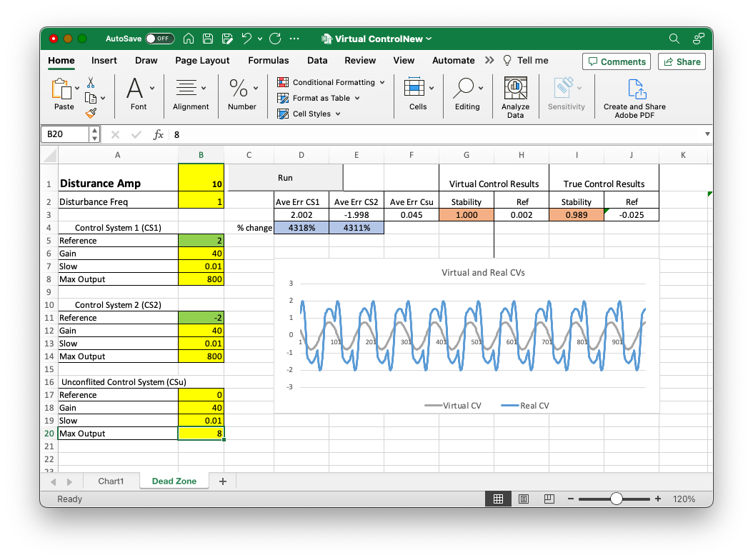
The spreadsheet opens to this display:


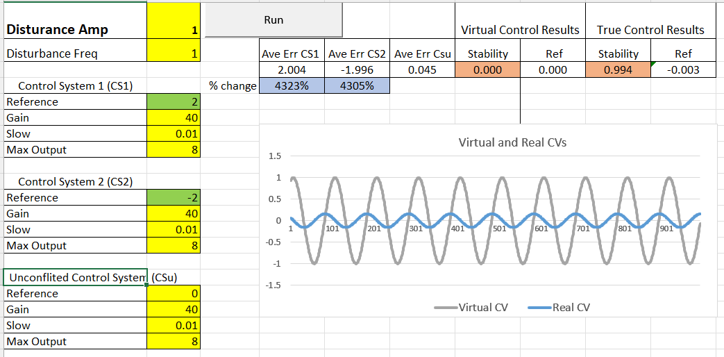
On the left, highlighted in yellow and green, are cells where you can enter values for the amplitude and frequency and frequency of the sine wave disturbance, and parameters for two control systems that are in conflict (CS1 and CS2) and an equivalent unconflicted contol system (CSu). The control systems are controlling the position of the same cursor in a tracking task; so the controlled variable is the same for both systems: cursor position.

To begin using the spreadsheet start by leaving all control system parameters as they are. The control systems are set to have equal strength in terms of Gain and Maximum Output. The conflicted control systems (CS1 and CS2) have references of 2 and -2, respectively, and the unconflicted control system (CSu) has a reference of 0, which is equivalent to the virtual reference of the two conflicted systems. . The disturbance is a sine wave with amplitude set to 1 unit and a frequency of 1 Hz.

Pressing the Run button simulates a 10 second run where both the two conflicted control systems and a single unconflicted control systems are controlling the position of a cursor under exactly the same conditions (the same disturbance). The results of that run, which are produced nearly instantaneously after pressing Run, are shown in the upper right of the display.

The most important results are the ones in light red – labeled “Stability” – which are measures of how well the conflicted and unconflicted control systems controlled the cursor. The stability measure (S) is calculated as:

S = 1 - sqrt(Var(C)/[(Var(D)+Var(O)])

Var(C) is a measure of the observed variance of the cursor; Var(D)+Var(O) is a measure of the expected variance of the cursor – expected if there were no control. To the extent that there is control the observed variance of the cursor will be much smaller than its expected variance and the Stability measure, S, will be close to 1.0. When there is no control the observed variance of the cursor will be equal to its expected variance and the stability measure will be 0.0.

The display above shows the results of a run with the disturbance amplitude set to 1. In this case the Stability measure for the conflicted system – the Virtual Control Results – is 0.0 while that for the unconflicted control system – the True Control Results – is .994!! So the conflicted control system was not resisting this disturbance at all - it was not controlling – while the equivalent unconflicted control system was resisting teh disturbance quite well – it was controlling nearly perfectly. This is shown in the graph below the results. The grey line shows that the cursor that is “controlled” by the conflicted control systems moves exactly in synch with the 1 unit disturbance while the blue line shows that the effects of the distrubance on the cursor were considerably attenuated by the actions of the unconflicted control system.

What you are seeing here is a complete lack of control by the conflicted control systems when the amplitude of the disturbance is in the Dead Zone. You are also seeing that there is no Dead Zone for the unconflicted (actual) control system – it acts to resist the same disturbance and keep the cursor under control.

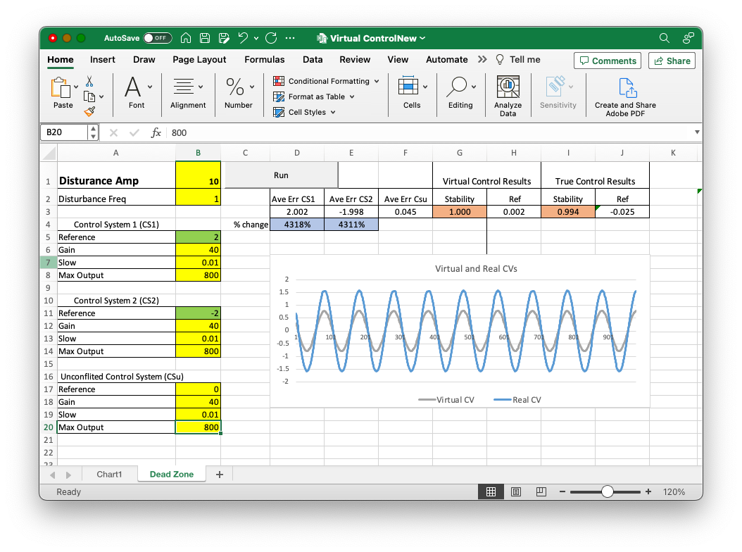
You can now use this spreadsheet to estimate the width of this Dead Zone by doing runs with varying values of disturbance amplitude and see which ones result in no control (Stability = 0.0) and which ones result in some amount of control (Stability>0.0). I’ve found that the Dead Zone for the conflicted systems of the strength entered into the spreadsheet (Gain = 40, Max Output = 8) seems to range from disturbance amplitudes of just over 0.0 to about 2 (0.0 amplitude can’t be used because it results in a denomintor of 0 for the stability calculation). Once the disturbance amplitude gets above two, the Stability measure becomes non-zero, as shown below, for a run when the disturbance amplitude is 3:

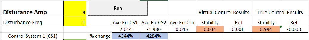
As you continue to increase the amplitude of the disturbance, the Stability measure for the conflicted control systems (the Virtual Control results) actually starts to increase; increased disturbance amplitude leads to better control! This is exactly the opposite of what happens with the unconflicted control system (the True Control results) where, as the amplitude of the disturbance increases, the Stability measure decreases; increased disturbance amplitude leads to worse control.

Thus, there are two ways to distinguish a virtually controlled variable – one controlled by conflicted systems – from a true controlled variable. A virtually controlled variable can be identified 1) by the existence of a Dead Zone where there is no resistance to disturbances with amplitudes in the Dead Zone range and 2) by the fact that increases in disturbance amplitude outside the Dead Zone range lead to increases in the ability to control the virtually controlled variable. For a true controlled variable there is 1) no Dead Zone and 2) increases in disturbance amplitude always lead to decreases in the ability to control a true controlled variable.

The above facts are true for a virtual controlled variable when the control systems "controlling’ it have equal Max Outputs. You can use the spreadsheet to see what happens when the Max Outputs of the two systems are unequal. I’ve done some explorations of what happens in this case but I’ll leave this for a separate post. For now, I developed this spreadsheet to see whether or not Bill Powers was right about the Dead Zone. And, once again, he was.

Thank you for this reply, Rick, but it has left me a little confused. Without yet having had the time to examine your spreadsheet closely (and perhaps you’ll send me a copy of the spreadsheet so that I can look at it more carefully), I have some questions about what you’re saying.

You start by reproducing Figure 6 from my 2004 paper, the simulation of conflict with limits on output, which I argued had not shown any “dead zone,” as Bill had predicted. Here’s what you say about it:

Bill described the dead zone as a range surrounding the virtual reference level, which I would take to refer to some range of values between +2 and -2, the reference levels of the two conflicting systems in your example. But you describe the dead zone as a “range of disturbance amplitudes.” What does you mean, exactly? Are you talking simply about a range of values that the environmental variable might take between +2 and -2 when affected by the disturbance, or are you referring to the range of maximum amplitudes of the sinusoidal disturbance curves that you tested in your example?

And why was my simulation not a proper test of the dead zone, however we’re describing it?

You go on to offer results from your own simulation of interaction between conflicted variables, giving each system a max output of 8. Is that a hard maximum, so that if the output can’t go any higher than 8 (in absolute value, I presume)? Why did you choose this very small value for the maximum output? It’s nowhere near the asymptote for the maximum output that the two systems with gains of 40 would exert in conflict with each other if they were free from any artificially imposed maximums. Checking my own spreadsheet, it looks to me like that asymptote is approximately 80 points in either direction, not 8.

It seems to me that your simulation here is a little like asking two people to play pingpong in a tiny room just barely big enough to accommodate the pingpong table. If they’re running into a physical barrier like a wall every time they go to make a shot, we might not be surprised if their control in this contest is not very good.

Your demo looks impressive, but I have a suspicion that there’s less here than meets the eye.

I have some other questions, but that’s probably enough for the moment.

Kent

Hi Kent
There was a link to the spreadsheet in Rick’s message:

Eetu

Hi Rick, thank you once again for your - as Kent said - impressive spreadsheet demo!
I am sorry to tell that I still cannot run those macros in my computer, but that does not much matter because the demo and your message are so informative anyway.
The Dead Zone is conceptually very clear: the effects of conflicting controllers cancel each other and neither can increase its power, so they can do nothing to the disturbances in the Dead Zone. But problematic is the practical consequences of this phenomenon. First I was concerned about the possible differences between a necessarily simplified abstract and frictionless model and a physical real world situation. I currently cannot do tests about this so I will not return to it now.
Two interesting points about or from the demo:
You said the control of the virtual controller gets better the greater the disturbance is (outside the Dead Zone). That supports my earlier claim that the collective control even if conflictual is or can be more profitable to the singular controllers than individual control if the disturbances are strong enough.
Secondly it seems that the Dead Zone is about half of the difference between the references of the participant controllers. What is the practical bearing of this zone to them? Quite minimal, I think. The different scale between your and Kent’s models may be somewhat deceitful.

Best
Eetu

Hi Kent

There was a link to the spreadsheet in Rick’s message:

Eetu

Happy to answer your questions. Eetu pointed you to the spreadsheet. You have to run it in Excel (rather than on the web) with macros enabled because the calculations are done in a VisualBasic macro. If you get far enough so that you can press the Run button and have the macro run with different input values for the disturbance amplitude I’ll show you how to get to the program itself.

The spreadsheet is initialized to have a Dead Zone ranging from +2 to -2, the reference signal values of the two conflicting control systems. What this zone is “dead” to are disturbances whose amplitude is between those two references.

In the first display in my previous post the disturbance amplitude was 1, which is within the Dead Zone, and the conflicted control systems did not resist this distrubance, as evidenced by the Stability value of 0.0. The same disturbance was resisted by the equivalent unconflicted control system, as evidenced by the Stability value of .994.

In the second display in that post the disturbance amplitude was 3, which is outside the Dead Zone (-2 to 2) and so there was some resististance, as evidenced by the Stability value of .634. The Stability of the unconflicted control system with this disturbance was the same as with the 1 unit distrbance, .994.

If by environmental variable you mean the disturbance variable then, yes, the Dead Zone is a range of disturbance amplitudes that will not be resisted by the conflicted control systems.

Because it doesn’t show that there is no resistenace to the disturbance when the amplitude of the disturbance is small enough, which means within the range of the references for the controlled variable – the Dead Zone.

I was having trouble figuring out why I was getting bad results with a Max value of 40. I have now figured it out and the spreadsheet that is now on line has a default Max value of 40 for all systems. But you can change those values to anything you like to see what happens.

It’s actually like having two people control the same cursor with a very weak disturbance. It would be nice to actually run such a task and see how well the model fits the data.

Actually, there’s even more that meets the eye. For example, I also present the % change in the amount of error experienced by the conflicted control systems compared to that experienced by a equivalent unconflicted control system (CSu). The % increase in error experienced by the conflicted systems relative to the unconflicted system is over 500,000% when the disturbance is in the Dead Zone.

Of course this is only true when the systems have different references for the value of the controlled variable. If you can get the systems to adopt equal or nearly equal references, you have cooperation and the systems have less error than they would have when working alone.

Great. Keep 'em coming.

I’ve had a chance to play around with Rick’s demo a little bit now, and it is as I suspected: the “dead zone” effect that the spreadsheet supposedly demonstrates is entirely an artifact of the imposition of arbitrary limits on the output of the pair of conflicted systems. If you take those artificial limits away (or make them a lot larger), the dead-zone anomalies disappear, too.

These limits on output are like setting up a tug-of-war contest with a wall erected directly behind each team, so that when they begin to pull the rope in their direction, the guy in the back immediately runs into the wall. Under those conditions, the team’s control won’t look to good. Or for an arm-wrestling contest, an artificial limit on output would be like attaching a straps to the contestant’s arms that prevented them from reaching palms-down all the way to the table. Physical restrictions on one’s range of motion interfere with control. In all the examples that Rick talks about, the limits on output interfere with the range of motion of the conflicted systems but not of the system working on its own. When you start removing those limits, things change.

In this example, I increased the limits on output for the conflicted systems to 800 but left the output limit for the lone system at 8. Because the amplitude of the disturbance has been increased to 10, the lone system is running into problems with hitting its output limit, causing the strange curve for the “Real CV” the environmental variable associated with the single system, and the stability measure is now higher for the conflicted pair than for the single system.

In this example, I’ve jacked up all the output limits so that none of the systems is encountering any arbitrary restriction on its movements. The stability indices are about the same, with the “Virtual Control Results” slightly better, and you can see the superiority of the control produced by the two conflicting systems, because the amplitude of the curve for the “Virtual CV” is just half that of the “Real CV”. The collective control produced by two systems with the same gain is twice as good as that produced by a single system of that gain, whether or not the pair of systems is in conflict (as I’ve repeatedly been saying).

This came as quite a surprise to me because there was nothing in Bill’s description of the Dead Zone to suggest that its existence was contingent on the limits of the output. So I spent the last two days trying to figure out why this happens and I’ve finally figured it out. Indeed, the existence of the Dead Zone does not depend on the output limits; you can make the output limits as high as you like and the Dead Zone still exists. This fact is demonstrated in a revised version of the Virtual Controll spreadheet which is available here.

Before I go over the spreadsheet I want to apologize to Kent because the reason he found what he did was all my fault. There was a flaw in the spreadsheet. The flaw was in my computation of the Stability Factor, which measures the quality of control. When disturbance amplitude is in the Dead Zone the Stability Factor should be 0.0. This was true when the maximum output was low (40). But, as Kent found, it was not true when the maximun output was increased considerably (by a factor of 20 in Kent’s example).

In the spreadsheet Kent used to make this finding, my computation of the Stability Factor failed to take into account the fact that, the greater the maximum output of the conflicted systems, the longer it takes those systems to reach their maximum output.

Recall that the Stability Factor, S, is computed as:

S = 1 - sqrt(var(CV)/ [var(OutputCS1)+var(OutputCS2)+var(d)]

In the program Kent used, I measured the variance (var) of these variables over the same fixed interval, regardless of the maximum set for the outputs of the two conflicted systems (OutputCS1 and OutputCS2). The result was that the measures of variance of the outputs were much greater when maximum output was high (800) relative to when it was low (40). This is because the interval over which I computed the variances included the changes in output that brought the high maximum output systems to their maximum. (Why this happened will become clearer when we look at the new spreadsheet). The result was that the denominator on the right of the the Stability equation --[var(OutputCS1)+var(OutputCS2)+var(d)] – was artificially large, resulting in a Stability value near 1.0, suggesting that there was nearly perfect control when, in fact, there was no control at all. When the maximum output value was relatively small, the variance of the outputs of the conflicted systems was 0.0 (since the systems were at a constant maximum), correctly showing that there was no control in that situation.

So the apparent disappearance of the Dead Zone with an increase in maximum output was a result of the program calculating the Stability Factor incorrectly. The new Virtual Control spreadsheet corrects this problem and shows that the maximum output limit has no effect on the exitence of the Dead Zone. It also shows that there is only control of the “virtually controlled variable” when the amplitude of the disturbance to that variable is greater than the range of the Dead Zone.

Here is what you’ll see when you open the new Virtual Control spreadsheet:

The sheet is pretty much the same as the prior one. I’ve mainly changed the starting system parameter values. All control systems now have a Gain of 90 and a starting Max Output of 1000. The Dead Zone range is the same as before – between references of 2 and -2 for the conflicted systems. And the disturbance is set to an amplitude that is within this Dead Zone.

There is a new item in the list of parameters labled “Start Vector” and it has a current setting of 3000. The meaning oif this parameter can best be seen by taking a look at the graph that shows the time course of the output variations of the two conflicted systems, CS1 and CS2. The variations range over 10,000 sample values representing 1 minute and 40 sec of interaction between the systems. The graph shows the variations in output of the two opposed systems when their maximum output is set to 1000. Notice that it takes about 750 samples (~12 sec) until the systems flatten out at their maximum output,1000.

It’s only during this flat section of the outputs, when they are at their maximum values, that the Stability Factor should be calculated. In order to do that you have to be sure that the calculations start at or slightly after the point in the data vector when the outputs have reached their maximum. The Start Vector parameter let’s you do this.

The Start Vector is currently set to 3000 because this places the start of the analysis window comfortably in the maximum output section of the data vector when the Max Output is set anywhere from 5 to 5000. If you want to see that the Dead Zone still exists at Max Output values greater than 5000 you will have to look at the graph and see where the outputs reach their maximum value and reset the Start Vector parameter appropriately.

You can use the spreadsheet to demonstrate to yourself that no matter how large the maximum output value for the conflicted control systems, there is no control (Stability = 0) as long as the amplitude of the disturbance if within the range of the Dead Zone. As you increase the disturbance amplitude beyond this range you will see that control begins to improve and eventually becomes comparable to that of the unconflicted system system results (Stability Factor close to 0.99). The fact that control improves with increasing amplitude of a disturnace is another way to distinguish a virtual from a real controlled variable since the latter shows a decrease rather than an increase in it’s ability to control (measured by S) with increases in the amplitude of disturbances.

One interesting discoverly I made with this spreadsheet is that the time (number of samples) it takes for the conflicted systems to reach their maximum value is inversely related to the size of the Dead Zone – the difference between system references; the larger the Dead Zone, the faster the conflicted systems reach their maximum values. Apparently the Dead Zone acts like a narrow band filter with respect to variations in the outputs of the conflicted system. Thus, the model makes an interesting (and testable) prediction about behavior in conflicts. If the parties to a conflict are asked to have references that differ by increasing amounts we should an increase in the speed with which the parties reach their maximum outputs.

There are many other interesting things that can be learned about the PCT model of conflict from this spreadsheet. But I’ll leave that for later. For now, if you are interested in this stuff, feel free to play around with the spreadsheet and I’ll be happy to answer any questions you have about it and I welcome whatever suggestions you have for further development of this model.

And for those of you who are intrested in how the program works that simulated the systems in conflict here is a copy of the Visual Basic program that does the simulation and computes the results.

Hi all,

First a small note about the earlier discussion in this thread about Kent’s data and diagram (2004) that it does not test or support the existence of the dead zone. I would say that it shows as a small hint in the end of the data that there is a dead zone but it can also show how insignificant the dead zone phenomenon may be. I did two additions to the diagram: a red oval to show where the dead zone phenomenon is visible and two thin red lines to show approximately the size of the dead zone (a half of the difference between the references of the individual controllers - actually the lines seem to show it somewhat too broad).

In PPC there is lengthy discussion about the phenomenon of a tolerance zone which is used in technical control devices and very probably exists also in living control systems because “It can improve the ability of a control loop to react rapidly but stably to a sharp change in reference or disturbance value (vol.1 p.115).” It seems to me that the dead zone behaves similarly as the tolerance zone and by TCV it would be impossible to see whether a variable is controlled by a virtual controller with a dead zone or an individual controller with a tolerance zone.

So I would ask you Rick if you could add an adjustable tolerance zone to the individual controllers in your demo and test then two things:

  1. How does the behavior of a variable differ when it is controlled by a controller with tolerance zone or by a virtual controller?
  2. What happens to a dead zone if the conflicting controllers have a tolerance zone?

And a third question: Is the dead zone always (just or about?) half of the difference between the references or does it depend on other things too?

Thanks
Eetu

I said that Kent’s model data did not test for the existence of a Dead Zone; Kent said that his data did not support the idea of a Dead Zone.

The behavior of the controlled variable (a segment of which at the end of the data is what you circled on the graph) has nothing to do with the definition of the Dead Zone. The Dead Zone is defined by the highest amplitude of disturbance that is not resisted by the systems in conflict. It turns out that that amplitude corresonds exactly to the distance between the references of the conflicted systems.

What’s PPC? I’m a B:CP man myself. And I have never seen any evidence that there is a tolerance zone in the control systems that produce the behavior of living control systems.

Sure, But it might take a while.

The Dead Zone is always exactly the total distance between the references of the conflicted systems.

OK, I was wrong because I trusted too much in your earlier message where you said:

And there the distance between the references were 4. Actually that fits well with Kent’s diagram because (if I now look more carefully) the other controller lessens its output exactly when the disturbance crosses over that controllers reference. So it seems that when the disturbance is between the reference levels it is not cancelled by the outputs because the outputs can cancel only each other.

Powers of Perceptual Control

That is strange. For me there are many variables which have a tolerance zone. One simple example is the saltiness of the food. If there is much too little salt then I can ask to add it. If there much too much then I cannot eat. But there is a certain distance between these values where I can eat my portion with content. Similarly I can tolerate certain amount of bad manners, disorder of my desk, and wrong politics. Tolerance make life easier for every one. I recommed :smile:.

Oh, no hurry at all!

Thanks and best,
Eetu

Yes, I said that before I was reminded (by Kent, I believe) that Bill had said that the Dead Zone was defined by the difference in the references between the conflicted control systems. My latest spreadsheet model demonstrates this characteristic of the Dead Zone more clearly.

Yes, you can see the Dead Zone very clearly in Kent’s diagram. Note that the disturbance often goes outside the range between the references, indicating that the disturbance amplitude was outside this range. That’s why you see what you describe. If the distrubance had varied within the range of the difference between references you would have seen the outputs of both systems flat line, as they do in my spreadsheet when the amplitude of the disturbance is within the range of the difference between references.

Subjective experience is not necessarily the best guide to understanding your own behavior. For example, the examples you give of your subjective experience of tolerance zones could actually be the result of low gain control or an internal conflict with a Dead Zone.

I said that I had never seen any evidence that there is a tolerance zone in human controlling based on my experience of modeling human controlling. I always got remarkably good fits to data – accounting for well over 95% of the variance in the behavior – using control models that had no tolerance zones. And the one time I did use tolerance zones the result was a poorer fit than a control model sans tolerence zone (see Figure 6 in this paper). Ironically, the data I analyzed in that paper was provided to me by the author of PPC, who wanted me to test his “threshold” model, which is a control model with a tolerance zone defined by threaholds around the reference value for the controlled variable. Apparently the results of my modeling efforts had no impact on his belief in a tolerance zone, proving once again the truth of the slogan Bill saw as a child in an embroidery hanging on the wall of his Aunt’s house : “A person convinced against their will is of the same opinion still” (edited to eliminate the casual sexism of the original).

Best, Rick

I don’t think Eetu is referring to thresholds around the reference value for an individual controller. After all, the topic here is collective control.

In an individual controller, a notion of ‘tolerance’ correlates with loop gain. The controller continues efforts to reduce error to zero, but not quickly enough to keep up with varying disturbances or forcefully enough to bring error entirely to zero. From the observer’s point of view, this can be represented as a circle around the reference value in x/y coordinates.

In collective control ‘tolerance’ is much reduced because it is the intersection of the separate circles of the participating individuals relative to the collectively controlled aspect of the public environment.

Conversely, the collective error function is the average of the individual errors, but the collective output is the sum of the individual outputs.

Consequently, a maverick may control a disparate reference value with high gain but little effect.

This is discussed in PPC vol. 3.

Yes, the topic is collective control, but individual controllers’ possible tolerance zones can affect the dead zone phenomenon. At least in this simple and somewhat unrealistic one-dimensional model where two controllers have different references for same variable and where the controllers cannot increase their output. There the possible tolerance zones would decrease the dead zone - make it narrower, and thus make the virtual control better. At least it seems so to me.

Individual tolerance zone may perhaps be connected to many other phenomena: low gain, internal conflicts, form of comparator function etc.

And, sorry another deviation from the topic:

I remember that there has been talk about a table where we should collect different controlled variables. What is its status and where it is? I suggest that Rick and others would put their experience there and list all the controlled variables they have modeled - with possible references to publications.

Thanks and all the best,
Eetu

Actually, the topic here is whether Bill was right about the existence of Dead Zones in two person conflicts like the ones modeled by Kent, who said Bill was actually wrong; I developed the Virtual Control spreadsheet to test this and it turns out Bill was right (as usual). By the way, the spreadsheet has now been revised so that it can correctly test for the existence of the Dead Zone between any two reference values. The previous version worked only if the reference values were symmetrical around 0.

Are you using “collective control” as a synecdoche for conflict or are you saying that this is true of all controlling that involves multiple individuals, such as the collective controlling modeled in BIll’s CROWD program? And how do you know that “tolerance” is much reduced in what you call “collective control”?

Again, is this true of all examples of what you call “collective control” or is it just true of interpersonal conflicts?

And everyone involved in a conflict will have no control at all when disturbances fall within the Dead Zone, which can be quite wide if the references of the systems involved in the conflict are quite far apart.

In Chapter 8 of The Study of Living Control Systems (SLCS) I described Bill Powers’ vision of what research aimed at testing PCT might look like. A major part of that vision was the development of a database of controlled variables, some identified by formal testing for controlled variables and others simply based on naturalistic observation of variables that seem to be maintained in reference states, protected from disturbance. The latter can be used as a basis for formal research aimed at getting a more precise description of the variables organisms control.

The status of this project is pretty much where it was before SLCS was published. The current version of the database is here. You and anyone else interested in PCT is encouraged to add to the table. I think doing so would be a good exercise in developing “control theory glasses” – the ability to see the phenomenon that PCT explains: control.

I’ve pretty much put in all the controlled variables that I’ve discovered through my research and demos. I hope you and others will give it a try now. Let me know if you do.