* Diagram Police *

This is going to be a little rant about diagrams, for nitpicky people. Diagrams are important for representing systems and understanding how they behave. A good diagram follows consistent rules, has a direct correspondence to equations or code associated with it. Diagrams in PCT are supposed to be more like engineering block diagrams, or analog computer setups, and not just lumps of boxes and arrows. Bad diagrams can generate confusion and misunderstanding.

So, here is one inconsistent diagram, not following its own rules set in the description under the figure.

This is from one of Bill’s introduction to PCT texts. He says in the description: Loop functions are shown in gray. Variable names are inside circles, and a text box describes what they represent.

The problem here are two extra functions NOT shown in gray. One in the Disturbance function that takes in D and outputs Kd * D, and more importantly, the adding function taking in Kr * Qo and Kd * D, which is simply written under the feedback function.

All good in the upper part. The environment should look something like this:

image

The comparator inside the system has its own box, why not the adder too? It is clearly an adder in the formula.

This is a good diagram, from LCS III, live demo:


I think something in the graphics is hidden, there should be a circle where the feedback quantity and disturbance meet. Every variable has a name, a line with an arrow, and numerical value. Every function has parameters and a box. Well, except for the ADDER, but at least there is an empty space for it (or a circle), and there is no disturbance function like above.

Here is an old diagram from DEMO2, Bill’s PCT tutorial. I think it is not consistent. Inside the system boundary, there are three functions, named above the diagram as Perception, Comparison and Action. Lines are variables, functions are in boxes.

image

In the environment, quantities are in circles, the feedback function and the disturbance function are in boxes, and lines are what exactly? It is not clear at all. Functions are represented with boxes both inside and outside - there should not be any difference between representation of variables in the system and outside.

Here is how I made that diagram in the reproduction of DEMO2 a few years ago:
image

The only difference is where the qo, qi and d are placed, I think that makes it clear that lines are variables. Looking at it now, I would loose the circles for qo and d, and maybe replace the comparator with a circle too, because they have no clear purpose in the diagram. the d circle could possibly by a generator of smoothed random signals.

Another one of mine, from a few years ago:

image

The t (tau) is representing a delay element, ok. The triangle has a parameter Kp and a reference signal, but the reference signal is not marked, so not good. It is supposed to be a comparator and an amplifier: x(t) = Kp * [ r - p[t-tau] ], and then the Kd is supposed to be a leak parameter for a leaky integrator, qo[t] = qo[t-1] - (x[t] - Kd * qo[t-1])*dt. There is an adder in the environment as a black circle, adding qd and qo; well, subtracting them, so it is another comparator, but has a different symbol than the comparator-amplifier triangle. Not sure why the variable names are ‘floating’ above lines. Also the leaky integrator symbol is the same as the adder/comparator on the left. Not very good.

Today, I’d probably make something more like one of these two:
image image

Could have some improvement in the delay element, it could also be a generic input function box, but this one has all the variables and function parameters.

Good critique.

In Bill’s Figure 1, he promises only to put loop functions in gray boxes. The disturbance enters the loop from outside so the disturbance function is not a loop function in the intended sense. In the same way, the function that produces one reference input “from higher systems” (plural) is not explicitly called out. As you say, the adder is not represented by a box and it is a loop function. However, the adder is properly part of the environmental feedback function. The formula is separately called out only because that part of the environment that the experimenter is manipulating as a disturbance is called out separately.

BN: However, the adder is properly part of the environmental feedback function.

Ok, fair play. I’d reserve the name “feedback function” for Qf = Kf*Qo, but the “Environment” function in Demo2 (equation #1) is the lumped function Qi = Kf * Qo + Kd * d. This makes the diagram pretty nice and symmetric. Maybe the output function needs a bit of work. I don’t care too much for circles around variable names, but it is consistent.

image

1 Like

All of the relevant physics, chemistry, optics, etc. are in the environment feedback function.

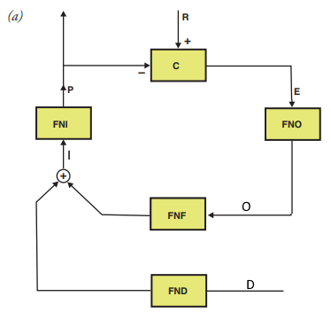
Here is another one, from Bill’s Byte articles from 1979. This one has an adder explicitly marked with a plus sign! But the I (input quantity) is next to it, not next to the line where it should be. And the circles for d and o are still here. Original and fixed:
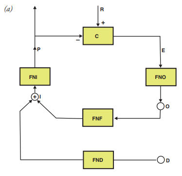
Byte diagram wrong Fix: Byte diagram fix

From 1978 spadeworks paper.

This diagram follows a different convention entirely. The lines with arrows are functions, while variables are ‘floating’. Again, there is no adding function in the diagram, but it is explicitly written in the text, qi = h(qd) + g(qo).

Not sure how to fix this. One way is to lump the environment into one function, and the other is to add the adding function and invent the notation. All the functions have one input and one output, so an arrow is easily representing that. If there are two inputs to a function, well, here is a try:

image
The diagram corresponds exactly to equations:
qe = h(qd)
qi = qe + qf
qo = f(qi)
qf = g(qo)


Another one:
image
Here, the equations are:
qi = env(qi, qo)
qo = f(qi)

env is defined as: qi = h(dq) + g(qo)

I prefer the first one.

edit:
image

image

This one is from Rick’s Controlled Variables: Psychology as the Center Fielder Views It, 2001.

There is one mistake and several inconsistencies. First, the mistake is defining the Feedback Function as “qi = g(qo)”. The Feedback Function is converting behavioral output to an effect on the input quantity. If the arrow is representing the function, the text under it should be qf = g (qo), or just g. If the intention was to define qi, the equation for this diagram would be qi = d + g(qo), but this equation should be written in a different place.

I’m really starting to feel bad for the poor adder getting left out of a lot of PCT diagrams. Adding is a function too!

The variables in the System are represented as lines with arrows, while outside there is one function represented as an arrow, one function missing (adder), and then one variable, d, represented as an arrow and two other variables represented as circles. Then there are two more unaccounted lines representing nothing; one going out from the output function; the other entering the input function. By convention set by the Feedback Function they are also supposed to be functions, but they are not.

So, two ways to fix this. One is to try following the convention that the Environmental variables are represented as circles, functions as arrows; but in the System, the variables are arrows, and functions in boxes.

image

Now it is consistent, but I don’t like it. The convention is changed between the System and Environment parts without good reason, in my opinion. Functions in boxes, variables next to lines:

image

Or lumping the Adder and Feedback functions into Environment function:
image


The following is from Warren’s and Rick’s The Origins and Future of Control Theory in Psychology (2015).

This is the engineering psychology diagram that the PCT diagram is supposed to correct:

image

And this is the incorrectly drawn PCT diagram:
image

The theme continues - inconsistent labeling of functions and variables, no adder.

The Controlled Variable is not a function as this diagram suggests, it is a function of one or more environmental variables (input quantities). The idiom “y is a function of x” means that both y and x are variables, and there is some function that takes x as input and gives y as output, y = F(x).

One possible fix:

image

There. Better.

Now, if the input function Yi is an identity function so that y(t) = p(t) then y(t) is also a controlled variable. If Yi is something like a differentiator or integrator, then the y(t) is not a controlled variable.

This one is great, from LCSIII, the mathematical appendix. Every function and variable accounted for, consistent notation, the adder is here, beautiful.

Only problem is that comparator is also an adder and the two adders are drawn differently?

They can be drawn equally, true! There is a slight ambiguity in the diagramed comparator - is the perceptual signal inverted or is it the reference signal? The function represented in a comparator is: F(a,b) = a + (-1) * b, Both functions can be represented as adders, and then inputs can have different signs for positive and negative (inverted sign), like the plus and minus next to an arrow in some of the diagrams up.

A similar scheme in B:CP:

image

They can also be drawn differently. Sometimes adders are boxes with the capital greek sigma [ Σ ], and comparators triangles with + and - input, like so:

image

but these might be confused with amplifiers which do comparison and multiplication and maybe low pass filtering.

It feels natural to mark p as negative and r as positive and then add them, as in http://discourse.iapct.org/t/diagram-police/15683/5. (Which should mean in LCSs that p is inhibitory signal?)

But isn’t it the same with environmental adder that output should cancel the disturbance and so they should have different signs? Here is a minimalistic one:

image001.png

(Now I no longer feel so much like a diagram criminal…)

The p signal is generally negative in the models and diagrams. If it is inhibitory or excitatory in terms of neural activity, I don’t know. There are only positive neural firing frequencies, and if inhibition is greater than excitation, there is zero output. I never quite got into trying to model those relationships.

Nice diagram! The environmental adder can be a comparator, but it could just add, too. Let’s say the reference is zero, and p = i. That means that if the control system is working properly, i will zero. If you have an adder in the environment, the equations is:
i = f + d ; inserting zero
f = -d

If you have a comparator, the equation is

i = f - d
f = d

or

i = -f + d
f = d

If you change the sign of f, then you need to change the gain of the output function from K to -K. If you have a comparator in the environment, then the output will be the same sign as the disturbance. If you have an adder, then it will be opposite sign.

Hi Eetu,

EJ: It’s my understanding that there needs to be an odd number of negative signs around the loop to preserve negative feedback. So I believe your inserting a negative sign at the environmental adder would remove the negative feedback.

Hi Adam,

Thanks for trying to clarify or clean up these diagram conventions.

EJ: You’re right that action potentials only propagate as positive frequencies in the nervous system. So to get bi-directional control (in either direction from zero) would require two different comparators. It’s like a rope: neural impulses can only pull.

EJ: This is what my presentation at the 2020 IAPCT Zoom Conference was about, showing structures for bi-directional control in the thalamus of the brain.

EJ: I don’t know yet how to create diagrams in Discourse, but I do wonder if our control loop diagrams should make this requirement clear. Maybe the comparator function box should be listed this way:
r - p


p - r

EJ: Inhibitory interneurons in the brain would be one of the standard ways of reversing the polarities.

EJ: You’re right that action potentials only propagate as positive frequencies in the nervous system. So to get bi-directional control (in either direction from zero) would require two different comparators. It’s like a rope: neural impulses can only pull.

Right, the important part of a comparator is that one signal is inhibitory and the other excitatory, producing a difference as the output; and then the total gain of the feedback loop is maintained negative by having different outputs from the two comparators, going in different directions.

For diagrams, I’m using https://www.diagrams.net/

EJ: I do wonder if our control loop diagrams should make this requirement clear. Maybe the comparator function box should be listed this way:
r - p

p - r

Yeah, I think if we are explicitly modelling or diagramming the neural implementation of a comparator, it should have both “types”.

I remember some other type of cell that was “inverting a signal”, Renshaw?

I followed this discussion loosely. I recognise that there may be many different purposes to use the basic PCT diagram but I also would like those adapted versions to refer to a basic loop.
I do think the diagram (* Diagram Police *) by Adam looks beautiful and could be used in PCT discussions more often. Could someone who’s on top of this discussion explain what the current state of the discussion is, and what others should consider when diagramming the basic feedback loop?

Hi Eva, thanks, feel free to use any of the diagrams I posted.

The important thing when making diagrams is to be consistent in the mapping between the math and the graphical part. If boxes represent functions, and lines represent variables, then this rule should hold in all parts of the diagram.

Basic functions are things like addition, multiplication, integration, etc, or they could be more complex, lumped into one box, like the ‘output function’ that contains multiple functions in it. Generally, functions have many input variables, but only one output variable.

Variables are, for example, the input quantity, the perceptual signal, the reference signal, etc.

1 Like

Here is one bad diagram. From the new book by Rick Marken.

This diagram seems to be following a convention where variables are letters, and functions are lines and arrows, but it is not consistent. The size of the spider, or as it appears on the screen, the distance of the spider from the participant is the CV. The CV should be S + R, and if arrows meeting on a variable imply addition (as in Bill’s diagram of the behavioral illusion), the dashed arrow should end on the spider. The function inside the head is maybe meant to represent the apparent organism function, but it has no place being in the head of the participant. The real organism function should be there. It is also a bit confusing what that head is doing, is it a variable like the R and CV, because it is represented by a letter, or a function because there are two arrows

Here is an improved version:

image

The letters are variables: S - stimulus or disturbance; CV - the controlled variable, size or apparent distance of the spider; R - response or output quantity of the participant, F - the feedback quantity, or the response multiplied by the feedback gain k.

The arrows are functions. The stimulus is acting on the CV through an unnamed function that doesn’t change the value of S. The addition function that creates the CV is marked explicitly above the spider. Then the head is supposed to represent the single organism function, here shown as pure integration (as opposed to leaky integration) for simplicity. The feedback function is the dashed line.

The behavioral illusion is thinking that the S-R function, R = -1/k * S is the organism function. Instead, the real organism function is shown in the picture of the head.

The diagram could still be improved, it is missing the reference value (Henry Yin would not be happy with PCT diagrams missing reference values).

Why the S-R function is equal to the inverse of the feedback function: if we assume the reference is zero, then we know that in a good control system CV will be equal to zero. This means that the F and S will be equal, but opposite sign, so that S + F = 0, or S = -F. Because F = kR, this means S = - k R and R = -S/k = -(1/k) * S, which is what the plot in the first image is showing.

Hi Adam

AM: Here is one bad diagram. From the new book by Rick Marken.

RM: I don’t think it’s “bad”. However, there is a mistake in it, so thanks for pointing it out. The feedback function equation at the bottom of Figure 1.4a should be CV = k R rather than CV = k S. The feedback function is correctly described in the text but I’ve contacted Cambridge U Press to see if there is any way to correct the error in future printings.

RM: Without this error I think the diagram is just fine. I think it makes the main point I want to make about the behavioral illusion, which is that it happens when the system under study is closed loop and and an observed relationship between a disturbance (S) to a controlled variable (CV) and the output (R ) that protects the CV from S is taken to reflect the organism function that relates S to R (the equation shown in the person’s head). That is, the illusion is taking the value of the coefficient relating the observed values of R and S to be a characteristic of the person when, in fact, it is a characteristic of the feedback function relating R to CV. This is shown pretty clearly in Figure 1.4b, where the subject seems a lot more sensitive to the approach of the spider in Take 1, with a weak feedback connection, than in Take 2, with a strong one. But it is not the subject who has changed; it’s the environment.

Best

Rick

The feedback function equation at the bottom of Figure 1.4a should be CV = k R rather than CV = k S. The feedback function is correctly described in the text

It is not correct, try asking Richard Kennaway, or check out his diagram in the math appendix of LCSIII.

image

The CV is the sum of effects of S and R, where R goes ‘through’ the feedback function to make the feedback quantity. Going back to your diagram:

Not correct:
CV = kR
CV = kS

Correct:
CV = S + k * R
or
CV = S + F and F = k * R

The feedback function is specifically the function multiplying R by k and creating the feedback quantity. The environment has another function, the adder for adding the stimulus effect and the feedback effect. The adding function is implied by two arrows ending on the CV (on the spider picture), but the feedback function does not involve the CV at all, so the CV should not be written under the dashed line representing the feedback function.

In the text, you say CV = kR, but this is never the case. The correct equation (always valid) is CV = S + kR. The function being inverted by the system is F = k*R.

the illusion is taking the value of the coefficient relating the observed values of R and S to be a characteristic of the person when, in fact, it is a characteristic of the feedback function relating R to CV

… relating R to the feedback effect on CV, not relating R to CV. But yes, that is the illusion, so it doesn’t make sense to me to put the wrong (illusory) organism function in the part of the diagram representing the organism in the control loop. The correct organism function would be more clear in its place because the high gain of the organism function explains why the F would be equal to -S, and why the inversion of the feedback function happens.