[I tried to reply from email but discourse cut the message from beginning. It is now corrected here.]
First I want to say that we are now discussing only the first (“preparatory”) part of Rick’s argument. I think it is no use to waste too much energy to this stage because the substantial grave error happens in second part. But the error begins already here.
I’ll attempt a paraphrase of what Eetu, Martin, et al. are saying. If it’s not actually a paraphrase, they’ll tell us, and you can ignore this, Rick, without responding to it.
Thank’s Bruce. for me it seems that you are at least nearly paraphrasing what I tried to say, but there are perhaps some unnecessary complications. Let’s see.
Richard Fineman famously advised us that “The first principle is that you must not fool yourself and you are the easiest person to fool.” I think these folks are saying that you are fooling yourself. The form of the self-deception is equivocation, taking two different things to be the same.
This is at least part of the diagnosis.
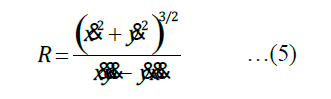
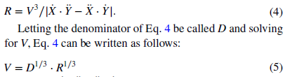
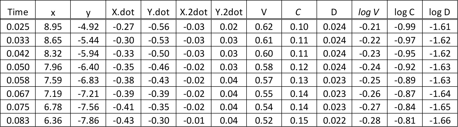
Everyone agrees that the V and R variables in (4) are instantiated with values of “the movement data” (Rick), “the measurement values” (Eetu) of particular movement paths. For each path, the relationship between V and R is given in the data, and a particular value of D can be calculated.
Yes.
According to Martin and Eetu and others the variables in (5) are not instantiated with any particular values because (5) is a generalization over all possible values of all three variables, V, R, and D. No ratio or proportion between V and R can be calculated from (5) unless D is held constant. (This is true generally of an equation with three variables, no?)
Yes, this is generally true of all this kind of three variable equations. We can know or infer something about the behavior of one or two variables if we know something about the behavior of the other variables. From this kind of strictly defined relationship between three variables we can infer nothing about the relationship between two of them if we do not know how the third behaves.
Holding D constant is kinda like instantiating D with data, except that values of D are not observational data. D is not observed as such, it is calculated from observed values of V and R. In (4), particular values of D are dependent upon and derived from particular observed values of V and R. In the different specific instantiations of V and R in (4), substituting specific measurements of velocity and curvature, D can have a range of values, and the proportional relation of V and R is variable.
D need not be necessarily held constant because it remains constant quite spontaneously IF the trajectory happens to obey the 1/3 power law (about the relationship between V and R). If the trajectory does not obey (or manifest) just that variant of power relationships between V (velocity) and R (curvature) then D is not constant but varies somehow.
When D is made a constant rather than being dependent upon the variable values of V and R, the proportional relation of V and R is constant. Making D a constant with some arbitrary value in (5) kinda looks like presuming the conclusion (petitio principii, ‘begging the question’).
I cannot say whether or that Rick thinks that D is always constant, because he admits that not all possible trajectories obey 1/3 power law. Rather he seems to think that there is some kind of “mathematical pressure” for all trajectories to come near that power law. But there is no (mathematical) mechanism which could create this kind of pressure. D has no privilege over other possible third elements in those kinds of three-part equations between V, R, and some third variable. Neither there is any metaphysical power or controller which would try to stabilize that D or any other third variable. D stabilizes if there happens to prevail that special power law relationship between V and R. And the question remains, why they behave so sometimes but not always?
 rsmarken:
In both cases [i.e. in both equation 4 and equation 5] they are computed from the X and Y values of the movement data
In (4), “the movement data” are data for a particular trajectory and D is derived from V and R; in (5), “the movement data” are all possible values of all three variables V, R, D and no constant proportion between V and R (or any pair of them) can be derived unless one of the three values is given a constant value. “All possible values” is a generalization.
Yes.
A finite set of observational data can be organized in a table Tn. Holding any one variable to a constant value excerpts a subset of that tabulation and in that subset the ratio of the other two values is constant. The values tabulated in Tn are not all possible values. The variables V, R, D in (5) ‘refer to’ imagined values in an imagined tabulation T∞ of all possible values for them. In imagined table T∞ the only way to get a constant ratio of any two values is by excerpting a subset of T∞ in which the third value has a fixed value.
For me this idea of observational table here feels like a complication, but it can be helpful for someone else.
rsmarken:
The variables R, V and D in both equations (the denominator on the right in equation 4 is equivalent to D) refer to measures of variable aspects of any curved movement (such as variations in the instantaneous velocity of the movement, V, over time).
“Refer to” has two meanings. In (4), the variables R and V ‘refer to’ the data for each trajectory, one at a time, and D ‘refers to’ these data indirectly, by solving equation (4) for those particular values. In (5), the variables R, V, and D ‘refer to’ ranges of observed values for R and V and calculated values for D. These may be imagined to be in a tabulation of all possible values, though in practice only a subset of all possible values are the observed data and the generalization of (5) enables unobserved values for two variables to be extrapolated from any stipulated value of the third.
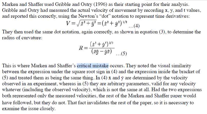
Yes, they refer in different ways in different stages – there happens quite of a metamorphosis. First the instantaneous values of R and V are determined in (2) and (3) based on the dotted (time derivative) values of x and y:


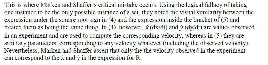
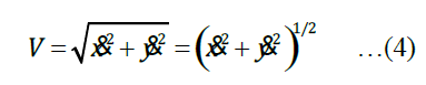
But then Rick thinks that contents of the brackets in in both equations are equivalent and replaces the bracketed part of (3) with D and gets the equations (4) and (5). However, as Martin said, these bracketed parts are not equivalent. It is perhaps not very easy to see their difference just by looking at equations. But think that (2) is a measurement of that current velocity and (3) is the measurement of that current curvature. Then note that the curvature is not dependent of the velocity of the object that is moving through it. The object can move through just the same curve with different velocities: you can drive the same bend of the road sometimes slower and sometimes faster. So the bracketed part – which is the velocity – is needed in (3) but it can be any velocity, not just that measured velocity of (2). Why seeing the difference between the bracketed parts of these equations is especially difficult to Rick, is that he thinks already beforehand that there must be some mathematical dependence between velocity and curvature – he needs it to show that power law research is pointless tinkering.
So the eq. (5) has lost its connection to the measurements of the original trajectory and it is valid for any velocity and any curvature – and as such tells nothing about the relationship between velocity and curvature, except if we happen to know that D remains constant.
Eetu