···
Bruce Nevin (2017.10.28.11:12 ET)
> o = k (r - p) where p = o + d so o = k*r + k*(o+d)
BN: Because it could be confusing, we should be clear that this is not a general formulation, but rather only for the case where r = 0 as stipulated for the proof in Bruce Abbott (2017.10.20.2015 EDT).
RM: Not true. The reference signal, r, is a variable.
BN: The expression (o + d) represents the net effect of output o and disturbance d upon aspects of the environment that are perceived as o.Â
BN: If d = 0 and o = 0 (no disturbance, so no output), for any value of r other than zero it is not the case that p = 0.
BN: The informal expression “no disturbance, so no output” expresses the inverse correlation between the disturbance and the output. Correlation does not entail causation. It doesn’t preclude it either.
RM: There are many problems with the expression “no disturbance, so no output”, not least of which being that it is wrong. If there were “no disturbance” (a phrase that only makes sense if it means “no effect of any variables on the controlled variable other than the system’s output”) there could still be output (which also only makes sense if it means “variation in the output variable”) due to variations in the reference specification for the controlled variable, r.Â
BN: In my view, this is not what is important. To deny that the negative correlation of output and disturbance is causation is rhetoric of the wrong kind.
 RM: I don’t think it’s rhetoric. It’s just a statement of fact; one of the most important facts about behavior that comes from PCT. What Powers (1978) showed is that the appearance of a causal relationship between disturbance and output in a control system has led scientific psychology astray since its founding as a discipline. It has led scientific psychologists to focus on studying these illusory causal relationships while ignoring the reason why these relationships exist - controlled variables.
BN: It is anti-persuasive rhetoric. Is there an arrow of causation between disturbance and output? Suppose there is. The important thing is that the arrow traverses a negative-feedback control loop. That recognition is cognitive jolt enough.
RM: The goal isn’t cognitive jolt; the goal is to explain why the study of living organisms should focus on describing the variables these organisms control, not on the variables that appear to “cause” behavior.Â
BestÂ
Rick
/Bruce
–
Richard S. MarkenÂ
"Perfection is achieved not when you have nothing more to add, but when you
have nothing left to take away.�
                --Antoine de Saint-Exupery
On Mon, Oct 23, 2017 at 11:20 PM, Richard Marken rsmarken@gmail.com wrote:
[From Rick Marken (2017.10.23.2020)]
Bruce Abbott (2017.10.23.0920 EDT)–
Â
BA:   Two points: (1) It is not true that if my sequential analysis were true, “then the correct equation describing the relationship between disturbance and output in a control system would be o = f(d); (2) The only variable affecting o in equation o = g^-1(d) is d, which proves my point that when the reference signal is constant, d is the only external variable affecting o.Â
RM: Though I disagree, I’ll give you point (1). But not point (2). The “behavioral illusion” equation,Â
o = g^-1(d),
doesn’t say that d is the only variable affecting (causing) o. It says that d a variable that is not affecting o. The function g in that equation describes the causal connection from o to the controlled input, q.i, as in,Â
q.i = g(o)
The inverse of this equation describes the causal connection from q.i to o – a causal connection that does not exist (the direction of causality goes from o to q.i). So the observed relationship between d and o is a correlation that does not imply causality. The correlation between d and o exists because of the way causality works when it is organized into a negative feedback loop. Powers (1978) showed that when causality is so organized, there will be a relationship between d and o but that relationship is not a causal relationship but rather, a *side-effect of the operation of causality in a negative feedback loop. *And the observed relationship between o and d will be an approximation to the inverse of the function relating o to q.i, the goodness of the approximation depending on how well q.i is controlled.
RM: What this means, of course, is that the observed relationship between d and o really tells us nothing about the nature of the organism under study. The observed relationship between d and o doesn’t “conceal” the true causal path from d to o; it doesn’t say anything about that path. You can’t “recover” that causal path -- the actual organism function – by taking the inverse of the inverse of the feedback function, for example. So any attempt to understand organisms by looking for relationships between variations in external events (independent variables) and the organism’s responses (dependent variables) – even if this relationship is looked for under controlled conditions -- will tell you nothing about about the behaving system under study. This is only true, of course, if the system under study is a negative feedback control system (N-system, per Powers (1978)); that is, only if it is a living system. This is the conclusion of the analysis in Powers (1978) and it is obviously pretty revolutionary and not something scientific psychologists particularly want to hear (or understand; to paraphrase Upton Sinclair “It’s hard to get people to understand something when success in their career depends on their not understanding it.”).Â
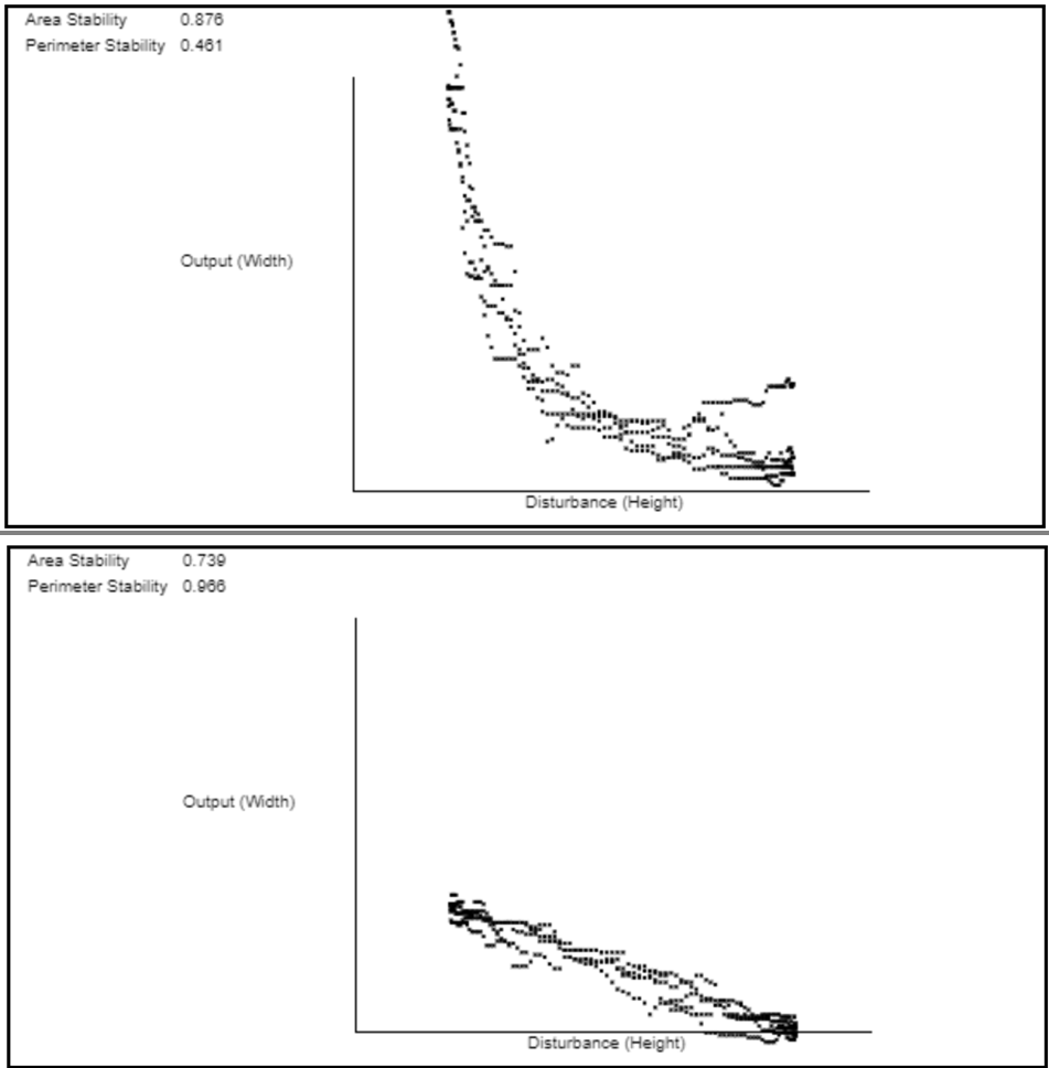
RM: The main things that looking at the relationship between d and o doesn’t tell you is that the organism is controlling some aspect of its environment, q.i, and what that aspect of the environment is. This can be illustrated using my “What is Size” demo (www.mindreadings.com/ControlDemo/Size.html). The graphs below show the relationship between d (the height of a rectangle) and o (width of that rectangle) in two different runs of the experiment. In the first (upper) run the function relating d to o appears quite non-linear; and, indeed, the relationship between o and d would be fit best by an equation of the form o = k/d. In the second (lower) run the function relating d to o appears to be quite linear; and, indeed, the relationship between o and d would be fit best by an equation of the form o = k-d.Â
Â
RM: From the experimenter’s perspective, nothing changed from the first to the second run; the d variable (height) is the same and the o variable (height) is the same yet we see two very different functions relating d to o. For some reason the causal path from d to o has changed for no apparent reason. If this were a real psychological experiment aimed at determining the relationship between d and o the inclination of the researcher might conclude that the “true” causal path from d to o is the average of these two results. But, of course, this misses the true reason for the difference in the shape of the relationship between d and o in the two cases. The difference is the variable that is being controlled, q.i.Â
RM: In the first run, the area of the rectangle was controlled and in the second the perimeter of the rectangle was controlled. This change in controlled variable – a change invisible to the researcher because it was made only in the mind of the behaving system – resulted in a change in the observed relationship between d and o because it changed the feedback connection from o to q.i. This is a change in the feedback connection which required no change in the physical link between o and q.i
RM: When area was controlled, q.i = o * d, which is the feedback function from o to q.i Since q.i was being held in a reference state, k, k = o * d and the inverse of this function o = k/d, same as the function that gives the best fit to the upper non-liner relationship between d and o. And when perimeter was controlled, q.i = o + d and since q.i was again being held in a reference state, k, so k = o + d and the inverse is o = k - d, again the same as the function that gives the best fit to the lower linear relationship between d and o.
RM: The point is that what is missing when you just look at the relationship between disturbances (stimuli) and output (responses) is the controlled variable, q.i, which is the link in “organism function” relating d to o. You have to know what an organism is controlling in order to understand why it acts as it does in the presence of certain “stimulus variables”. The revolution of PCT results from the “discovery” of controlled variables; the aspects of the environment around which behavior is organized. It’s controlled variables that have been left out of the explanation of behavior. It’s controlled variables that explain the observed relationships between stimulus and response variables. It’s these stimulus-response relationships that seduced psychologists into thinking that these relationships reveal something about the nature of organisms. Unfortunately, they are a red herring that has blinded psychologists to the most important fact about living organisms; they keep various aspects of their environment in reference states, protected (by variations in their outputs) from disturbances (which appear to act as stimuli).Â
BA:Â Having established the points I wished to prove, I am not going to engage with you further on this issue.
RM: I thank you for engaging as far as you have. You and Martin always give me good ideas for how to explain Bill’s truly revolutionary discoveries. I won’t engage further on this myself-- or at least I’ll try not to. But I will leave you with the final passage from what I believe is to be Bill’s foreword to LCS:IV, the book that he hoped would set out the new direction for the revolutionary new science of life based onPCT:
BP: The massive opposition [to PCT] from some quarters and
the passive resistance from others came as a disappointing surprise, but
perhaps it shouldn’t have. Science has a social as well as an intellectual
aspect. Scientists are not stupid. They can look at an idea and quickly work out
where it fits in with existing knowledge and where it doesn’t. And scientists
are all too human: when they see that the new idea means their life’s work
could end up mostly in the trash-can, their second reaction is simply to think
“That idea is obviously wrong.” That relieves the sinking feeling in
the pit of the stomach that is the first reaction. Being wrong about something
is unpleasant enough; being wrong about something one has worked hard to learn
and has believed, taught, written about, and researched, is close to
intolerable. All scientists of any talent have had that experience. The best of
them have recognized that their own principles require them to put those
personal reactions aside or at least save them for later. They know that any
such upheaval is going to be important, and ignoring it is not an option. But
those who recognize and embrace a revolution in science are the exception. Most
scientists practice ‘normal science’ within a securely established – and
well-defended – paradigm.
Â
BP: That is what we are up against here, and have
been struggling with since before most of you readers were born. We have spent
that time learning more about this new idea and getting better at explaining
it, but no better at persuading others to change their minds in a serious way
when their career commitments are threatened by it. What we had thought would
be a nutritious and deliciously buttered carrot has proven to function like a
stick. The clearer we have made the idea, the more defenses it has aroused.
Â
BP: We are now facing reality. This is going to be a
revolution whether we like it or not. There are going to be arguments,
screaming and yelling or cool and polite. It’s time to sink or swim. [Italics mine]
RM: Makes me think Bill really meant it when he said PCT overthrows the basis of scientific psychology.
BestÂ
Rick
Richard S. MarkenÂ
"Perfection is achieved not when you have nothing more to add, but when you
have nothing left to take away.�
                --Antoine de Saint-Exupery