[Martin Taylor 2010.01.08.16.54]
[From Rick Marken (2010.01.08.0930)]
Martin Taylor
(2009.01.08.00.35)–
2. How did you optimize the model fit?
Manually. I first fitted the model, with Kd=0, by finding values of
Gain and Damping that gave the smallest RMS error between model and
subject. Then I increased Kd. As soon as Kd>0 the fit of the model to
the actual behavior worsened (RMS deviation of model from actual
behavior increased).
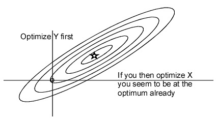
That isn’t a proper 3-parameter fit, is it? If you have optimized two
parameters with the third fixed, varying the third is almost guaranteed
to give worse results, except in the special case where the effects of
the third are orthogonal to the effects of the other two.
This is a good point. I have just tried fitting the model with all
three parameters – Gain, Damping and Kd – varying simultaneously. The
result is a 1% improvement in the fit when Kd is included in the model
as opposed to when Kd is set to 0 and only Gain and Damping are varied
(the way I did it before, so that the addition of Kd always makes
things worse).
I’m actually not sure what to make of this. The model sans inclusion of
the derivative in the input accounts for just about as much variance in
the human behavior as the model can account for. My guess is that the
1% reduction in RMS deviation (between model and human) that you get
when you vary 3 rather than just 2 parameters to fit the model results
from the fact that you now have more predictor variables (as when you
add a predictor variable in multiple regression). Given the extra
“degree of freedom” it seems to me that you are bound to increase the
amount of variance accounted for by the prediction equation. But if the
increase in variance accounted for by the increase in number of
simultaneous predictors (from 2 to 3, in this case) is very small (as
it is in this case, just an increase of 1%) the added predictor would
be discounted as being insignificant.
So the results of my analysis still suggest to me that humans do not
include the derivative in the controlled perception in a tracking task.
OK. I’ll agree with you about the added predictor, so we seem to be in
agreement that awake and alert subjects don’t use much if any
prediction when there is little or no “sluggishness” in the control
loop.
When you say “The model sans inclusion of the derivative in the input
accounts for
just about as much variance in the human behavior as the model can
account for.” how much is that, on average? It makes a difference in
how you view the 1%. If the non-predictive model accounts for 80%,
there’s 20% unaccounted for, of which the predictor accounts for 5%,
but if the non-predictor model accounts for 99%, then the addition of
the predictor accounts for all that’s left, making it quite important
to consider the effect of the predictor, small though it may be.
On looking now at the 14-year-old C code for my analysis of the sleep
study, I see that the way I optimized might not have been ideal,
either. What I did was to start by computing a best value for delay d
and then for gain k (as Rick did), and use those values, with
prediction z at zero, as a starting point for further optimization. The
continued optimization was done by getting the RMS deviation between
the human and the model track with the parameter values at d, k, z, and
vary each of d, k, and z by an amount determined from earlier steps in
the analysis, doubling or halving the step in each independently
according to the PEST procedure. I then determined a point with a new
d, k, z, by adding those newly calculated increments in each
dimensions, and another new d’, k’, z’ at the same distance in the
opposite direction (because simply stepping across the minimum diagonal
could be going in the wrong direction). Whichever of the new d, k, z or
d’, k’, z’ gave the better fit with the human track was taken as the
start point for the next move. The idea, I imagine, was to work with
the assumption that the landscape was smooth, and to find a direction
that aimed most directly at the optimum. I must have thought that would
work better than e-coli, but I don’t remember ever doing a comparison
to see which gave more consistent results.
Looking at the C code, here’s how I eliminated periods of the data that
seemed likely to reflect times when the subject was not tracking
“normally”, meaning that the model was not designed to fit those
periods. There were three kinds of “not normal” periods, microsleeps,
subject getting lost (perhaps another kind of microsleep), and
“bobbles” when the human’s tracking error was unusually great:
-
Eliminate “microsleep” periods. These were defined as periods in
which the mouse did not move at all for at least 1 second. Data within
a microsleep period were designated as having validity 0.
-
Compute the real tracking error sample by sample except for the
points already marked as not valid.
-
Mark as invalid those places where the subjects seemed “lost”,
defined as having either an error greater than half a screen, or having
a derivative greater than 1000 (pixels per sample period over 4 samples)
-
Eliminate “bobbles”, according to a suggestion by Bill P.: Eliminate
points for which the tracking error was greater than 4 time the rms
tracking error.
In running the model, no account was taken of these periods insofar as
the model continued running throughout, but in computing the RMS error
to determine the goodness of fit for a particular set of parameter
values, the “non-valid” samples were ignored.
Here’s the C code loop for running the model, after a lot of
initialization. I’ve added a few comments to help in its interpretation.
This seems to be the latest of several versions in the folder I
recovered, so I expect it is the one that was used in the reported data.
···
============
`for(j= -200;j<datasize;++j) /* Both human and model have a 200
sample run-in period before measures are used */
{
if (--m <= 0) m = 30; /* m is an index for a ring buffer used
to implement delays */
i = abs(j);

hdelay[m] = h + distsign * (float)dist1[i];  /* h is the output
variable (don’t ask why it’s h rather than “output”) */
/* hdelay will become
the perceptual value after dy + dfract samples */
p1 = hdelay[(dy+m)%30 + 1]; /* Assuming the delay is all
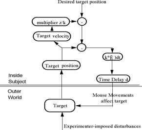
perceptual and not in the environmental feedback path! */
/* MMT comment 2010.01.10 This differs
from the diagram, in which the delay is
/* placed between the output and the
point where the disturbance enters the loop */
p3 = hdelay[(dy+m-1)%30 +1];  /* Added by MMT 950929 */

pz = p3*(1-dfract) + p1*dfract; /*MMT 950929 to centre derivative
on same moment as current perception */
/* MMT 2010.01.10 dfract is the
fractional part of the floating point
                                /* delay being tested on this run */

e = ref - p;

deltap = (pold - pz)/2.0;   /* pz is one sample time before p,

                            /* pold one sample time after p */

                            /* MMT 2010.01.10: This line looks like
a bug, since pz is the
/* perception at some fractional sample
time.
/* The divisor should presumably be
1+dfract, rather than 2.0
/* This bug should make the fits
noisier than they need be, since from one
/* model run to the next, the effect
could be similar to a change in z
/* by a factor of as much as 2, which
might well affect the optimization process */
h += k*e + z*deltap; /* pold and deltap added 950929 MMT *//* Here
is the output function */
pold = p; p = pz;

if (h > 1000.0) h = 1000.0;

if (h < -1000.0) h = -1000.0;

if(j < datasize && j >= 0)

  {

    modelh[j] = (short)h;

    u = (float)(modelh[j] - realh1[j]);

    if (valid[i]) {         /* MMT 2010.01.10 We avoid the
not-valid periods only when computing the RMS misfit */
/* I thought I had added a guard band
around each “not valid” period, but I see
/* none in the validity-setting code.
Perhaps they should be added if the old data
                            /* is to be reanalyzed */

      errsum += u;

      errsq += u*u;

    }

  }

}
errsq = errsq - errsum*errsum/validsize;
return errsq;
}`
============
I hope this helps in understanding just what was fitted to the data.
You will note that the integrator output function does not have a leak.
The leak rate would have been a fourth parameter in the fit. Maybe that
was a bad decision, but fitting four parameters offers more opportunity
for noisy interactions to affect the important parameters in the
optimization. With the extra compute power we have now as compared to
the mainframe I used in 1995, it should be possible to take four
parameters into account. In 1995, the fitting of three parameters to
over 400 tracks took rather a lot of computer time! I don’t know how
badly, if at all, the bug noted in the comments above would have
affected the published data, but if it did affect them, the effect
would have been to make them noisier than they should have been, and
making it harder for real effects to show up above the noise.
I haven’t got to the stage of trying to figure out how to go about
compiling the code, yet. But I think I’m beginning to understand it at
least a little. I used to write a lot of C, but I haven’t looked at it
since these studies, and reading the code Bill and I wrote at that time
is a bit like trying to read French after not having looked at French
for a decade. It comes back, but not immediately. Next I have to learn
what all the compiler flags must be, and how to interface with the
graphics. It might be easier to use the C code as a guide and rewrite
the whole thing in Ruby!
Martin