Fitting data to models

Martin_Taylor2 · August 7, 2005, 3:08am

[Martin Taylor 2005.08.06.21.15]

This may be premature, but I will be away until about August 30, so I'll report what I can at this point.

At the meeting, I made three presentations, on Layered Protocols, on the possible existence of social control systems, and on some issues concerning fitting data to models. I have uploaded the Powerpoint presentations I used to my web site, at <http://www.mmtaylor.net/PCT/index.html>. You can download them from there if you want (it might help make sense of this message to download the "Fitting Models" powerpoint).

One of my presentations was on fitting data to models. I have tracking data for 32 subjects, each doing seven tracks on each of six tasks of varying complexity, a total of over 1300 tracks. The six tasks were three controlling the perception of written number and three controlling the perception of line length. They are described more fully in the presentation, but here I should say only that there are three levels of complexity, which I call easy, medium, and hard.

As I mention in my presentation, I am testing two different five-parameter models, both of which often provide good fits. At the time of the meeting I had done about 60% of the tests with one model (model A in the presentation). That model has now been run on all the available tracks (it takes a day to test one subject's data).

The reason for this probably premature message is that before leaving I have managed to run two subjects on the other model (model B in my presentation) and have compared the quality of the model fit for the two models with those two subjects. Of course, it is never guaranteed that the genetic algorithm will discover the true optimum parameter values for either model on a given track, and as I discussed at the meeting, the fitting criterion itself is unlikely to be optimum. Given those caveats, I think the results for the two subjects are suggestively interesting.

Each subject has 21 tracks with the number perception. For the "easy' and "Medium" conditions, model B has a slight edge, but for the "hard" number condition model A usually gives the better fit (6 out of 7 tracks for one subject, 4/7 for the other). I cannot tell at this point whether there is any trend across complexity, because of the noisiness of the optima found by the fitting process. For the line length, model B gives the best fit most of the time (for the first subject 19 out of 21 tracks), usually appreciably better. Again, I can't yet tell whether complexity makes a difference to how much better B is than A for the line length task.

It will be interesting to see whether the trend holds up across more subjects for model B to fit better under most conditions, considerably so for the line length, but for model A to fit better for the "number hard" task. The effect could be a statistical anomaly due to the fitting process not always being able to find the best parameter set for the model, but I am inclined to think not. Another 15 subjects should be tested in my absence and all 32 should be done by the end of September.

It's slow going, but interesting.

Martin

Bill_Powers1 · August 7, 2005, 2:17pm

[From Bill Powers (2005.08.07.0751 MDT)]
Martin Taylor 2005.08.06.21.15 –
It was surprising how many people at the meeting, even non-technical
people, found your presentation interesting. I guess there is always
interest in hearing someone competent talk about doing something complex
and difficult.
In thinking over your project, I have come up with one definite opinion:
I don’t think you will get the best results by trying to fit one model to
all of the data, even in a single run. We talked a bit about this at the
meeting, but I am realizing it is more important than I thought
then.
In an experimental run where there are episodes of inattention, sleep,
instability, and so on, the basic premise of model-matching as an
analytical tool is violated. The model necessarily assumes not only that
a certain set of parameters governs behavior, but that the parameters
remain the same throughout the run. If that’s not true, then not only
does the model fail to fit the behavior as well as possible during the
anomalous episodes, it fails to fit it as well as possible between those
episodes, too.
It seems clear to me that the only solution is an iterative one, whereby
criteria are applied that divide the data into “normal” and
“anomalous” periods. The model is fit to the normal data, and
then it is used to estimate the changes in parameters during anomalous
intervals. By that I mean that the model derived from the normal periods,
with fixed parameters, is used to make a prediction of behavior during
the anomalous period, and then the difference is used to estimate the
values of the parameters during that period. This is the method I used,
without formalizing it, in the “Measurement of volition” paper
in Wayne Hershberger’s book. There are two overall criteria for selecting
the best model: minimum difference between model and real behavior during
normal periods, and minimum variations of parameters needed to achieve an
equally good fit during anomalous periods. It may not always be possible
to say which parameters should be changed – they may have
equivalent effects on total error – but at least an envelope of changes
can be determined. In my Hershberger paper, the experiment left only one
obvious parameter to determine, the reference signal, and the conditions
were deliberately changed during the anomalous period.

The object, of course, has to include eliminating as much of the data as
possible from the “anomalous” category, which means
experimenting with the classification criteria to maximize the amount
of"normal" data.

I don’t know if this experimental strategy has ever been formally stated
before. Do you know if it has a name?

Best,

Bill P.

Richard_Marken2 · August 7, 2005, 7:10pm

[From Rick Marken (2005.08.07.1210)]

Bill Powers (2005.08.07.0751 MDT) to Martin Taylor (2005.08.06.21.15) --

In thinking over your project, I have come up with one definite opinion: I don't think you will get the best results by trying to fit one model to all of the data, even in a single run.

Two other quick observations on this topic.

1. The results one gets when trying to fit models to data depends not only on the model(s) but also on the quality of the data. In statistical modeling (which I used in my thesis research) there is a concept of "predictable variance" which is the amount of variance in the data that is _not_ the result of unsystematic "noise" variance. I think this concept is relevant to modeling the results of control experiments because at least _some_ of the observed variations in such experiments are going to the result of "noise" -- slippage of the mouse, literal "noise" distractions in the room, etc. Event the fanciest parameter variation strategies won't help a model account for these kinds of variations. Unless you can figure out what level of fit is _possible_ for a model they won't know when the fit you've got is as good as the best fit you're going to be able to get.

2. When I start finding myself trying more and more subtle strategies to improve the fit of a model to data, I realize that I am acting like an obsessive gambler: I see myself thinking "I bet I can find a way to set the parameters so that I can get the average RMS error over subjects down from 18 to 15 cm, beating out the alternative model". When I "go up a level" and notice this addictive behavior, I realize that this "fitting game" is done in the service of a higher level goal: figuring out how behavior works. And the way to achieve that goal is not just to find good model fits but also to design experiments that will distinguish clearly between models. So once I see myself obsessing about model fitting, I realize it's time to quit doing that and to start trying to design a study that will help guide my modeling efforts -- experiments that will clearly expose the need (if there is one) for one kind of model or another. This is where I am right now on the catch modeling: it's time to stop trying to get minor improvements in the fit of my model relative to competitors and to start designing experiments that will better discriminate models that fit the data about equally well (though neither one perfectly).

Best regards

Rick

Richard S. Marken
marken@mindreadings.com
Home 310 474-0313
Cell 310 729-1400

Bill_Powers1 · August 8, 2005, 1:28am

[From Bill Powers (2005.08.07.1924 MDT)]

Rick Marken (2005.08.07.1210) --

Two other quick observations on this topic.

1. The results one gets when trying to fit models to data depends not only on the model(s) but also on the quality of the data.

In Martin's experiments, he had little to say about how the experiments would be conducted.

Unless you can figure out what level of fit is _possible_ for a model they won't know when the fit you've got is as good as the best fit you're going to be able to get.

Good point. I agree.

it's time to stop trying to get minor improvements in the fit of my model relative to competitors and to start designing experiments that will better discriminate models that fit the data about equally well (though neither one perfectly).

Going to try for some grant money? That would be an interesting direction to go in.

Best,

Bill P.

···

Best regards

Rick

Richard S. Marken
marken@mindreadings.com
Home 310 474-0313
Cell 310 729-1400

Richard_Marken2 · August 8, 2005, 3:20pm

[From Rick Marken (2005.08.08.0820)]

Bill Powers (2005.08.07.1924 MDT)--

Rick Marken (2005.08.07.1210) --

Two other quick observations on this topic.

1. The results one gets when trying to fit models to data depends
not only on the model(s) but also on the quality of the data.

In Martin's experiments, he had little to say about how the
experiments would be conducted.

I know. I didn't mean to appear to be criticizing the quality of Martin's
data. All I mean is that, in general, for any data, the goodness of fit you
can get is limited, to some (largely unknown) degree by random variations
(like the mouse slips I mentioned). This random variation may be quite large
(as it is in the typical psychology experiment, where models are considered
"good" if they pick up 30% of the variance) or quite small (as it is in
control experiments, where we can regularly pick up 99% of the variance in
some variables).

Unless you can figure out what level of fit is _possible_ for a
model they won't know when the fit you've got is as good as the best
fit you're going to be able to get.

Good point. I agree.

it's time to stop trying to get minor improvements in the fit of my
model relative to competitors and to start designing experiments
that will better discriminate models that fit the data about equally
well (though neither one perfectly).

Going to try for some grant money? That would be an interesting
direction to go in.

I have a hard enough time getting grants to do research (on healthcare
quality) that people are willing to pay for. I don't think I'd have much
luck getting money to study catching balls. I'm hoping that people who are
in a position to do the research I would like to see done will do it and let
me in on the data analysis.

Best regards

Rick

···

--
Richard S. Marken
MindReadings.com
Home: 310 474 0313
Cell: 310 729 1400

--------------------

This email message is for the sole use of the intended recipient(s) and
may contain privileged information. Any unauthorized review, use,
disclosure or distribution is prohibited. If you are not the intended
recipient, please contact the sender by reply email and destroy all copies
of the original message.

Martin_Taylor2 · October 11, 2005, 9:55pm

Re: Fitting data to models
[Martin Taylor 2005.10.11.17.18]

[From Rick Marken (2005.08.08.0820)]

Bill Powers (2005.08.07.1924 MDT)–

Rick Marken (2005.08.07.1210) –

Two other quick observations on this topic.

The results one gets when trying to fit models to data
depends

not only on the model(s) but also on the quality of the
data.

In Martin’s experiments, he had little to say about how the

experiments would be conducted.

I know. I didn’t mean to appear to be criticizing the quality of
Martin’s

data. All I mean is that, in general, for any data, the goodness of
fit you

can get is limited, to some (largely unknown) degree by random
variations

(like the mouse slips I mentioned). This random variation may be quite
large

(as it is in the typical psychology experiment, where models are
considered

“good” if they pick up 30% of the variance) or quite small
(as it is in

control experiments, where we can regularly pick up 99% of the
variance in
some variables).

Quite so. And I take your earlier point: " When I start
finding myself trying more and more subtle strategies to improve the
fit of a model to data, I realize that I am acting like an obsessive
gambler: I see myself thinking “I bet I can find a way to set the
parameters so that I can get the average RMS error over subjects down
from 18 to 15 cm, beating out the alternative model”

This is a problem of which I’m well aware. We all get caught in
it sometimes. I hope I’m not in that position right now.

I am in the position of having difficult data out of which
something interesting may come. It’s noisy for two reasons, perhaps
more. The two reasons are (1) the inconsistency inherent in having
sleepy subjects doing a task that is not of particular concern to
them, and (2) the inconsistency inherent finding the best
multi-parameter fit of a model when the form of the fitting function
is unknown and one has to use a randomized approach to the optimum
(the genetic algorithm outperforms e-coli, but it is still far from
guaranteed to find the best fitting parameter set for a given
model).

Given those two inherent reasons for noise in the data, I’m not
going to insist that results apply uniformly to every subject.
(Anyway, I believe that to be a wrong expectation in most
circumstance, but I won’t argue that point here. People can be
different, and that’s all I need to point out).

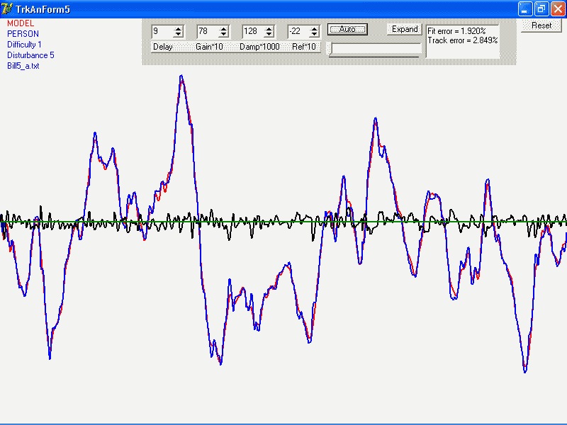
Now for the item of interest I discovered today. It’s embodied in
the graph I both attach to and embed in this message.

As you may remember, I’ve been doing a long-running program of
fitting two different models to some 1300 pursuit tracking runs, 42
from each of 31 subjects (there were 32, but one got sick and didn’t
finish the experiment. The data from that subject are totally
ignored). There were two kinds of tracking, one in which the target
was a two-digit number and the subject controlled another two-digit
number, the other in which the target was a line length and the
subject controlled the length of a different line. For each type,
there were three levels of complexity: “Easy”, in which the
subject equated the controlled value to the displayed target value;
“Medium”, in which the subject was asked to equate the
controlled value to the displayed target plus or minus a quantity that
was fixed for the length of the run; and “Hard”, in which
the subject equated the controlled value to the sum or difference of
the displayed target and another value that changed more slowly during
the run.

There was no attempt to balance the number of male and female
subjects in the study. Of the 31, 14 were male, and 17 female.

As I said, I’ve been fitting two models. At the CSG meeting I
called them “Model A” and “Model B”. In the graph,
they are “17o” and 18a" (which perhaps gives you an
idea of how many models have been tested in all). Both provide
reasonable fits to many of the tracks. Recently, I’ve been comparing
them track-by-track in two ways, the relative goodness of fit, and
simply which one gives the better fit.

When I looked at the first batch of subjects, it seemed quite
clear that the “17o” model was more likely to give the
better fit, but that this preference declined sharply for the
“Hard” conditions, both number and line-length (I call those
“numeric” and “graphic”). When I looked at the
second half of the subjects, this pattern was not there. I figured
that there might be something different about the subjects and their
ways of looking at the world, so I went back to the experiment logs to
see if I could find anything.

An obvious thing to check is gender. It turned out that most of
the subjects in the first batch were male, and most in the second
batch were female. So I looked at the pattern for each subject
individually, making one graph with 14 lines on it for all the male
subjects and one with 17 lines for all the female subjects. The two
graphs were quite different. One male subject had a pattern that would
have fitted better in the female group, and two females had patterns
that would have fitted better in the male group.

The next thing, which I finished a few minutes ago, was to take
the male and female probabilities that model 17o provided a better fit
than model 18a for each of the six experimental conditions. These are
averaged across all male and across all female subjects. I show them
the numeric and for graphic conditions separately. There seems to be a
clear difference between the sexes in how they deal with the
complexity of the task, and that difference is consistent between
number tracking and line-length tracking.

The main difference betweenthe models is that 17o compares the
(delayed) perception of the target value with the current value, and
uses that to set the reference for the difference between a (delayed)
perception of target velocity and the current cursor velocity, whereas
18a uses the (delayed) perception of the target velocity and the
(delayed) perception of the target position to produce a current error
value which is used to set a reference for cursor velocity.

I’m trying to think of a model I can parameterize that would
contain elements of these two models and that is psychologically
plausible, with a view to seeing if I can find a parametric shift that
makes sense and that suggests a link with other mental characteristics
differentiated by sex. But I’m off to a NATO meeting on Friday, and
won’t get to it until November. I thought I should give you this minor
progress report before I left.

Martin

ModelFits_Gender.pdf (16.3 KB)

Richard_Marken2 · October 12, 2005, 7:49pm

[From Rick Marken (2005.10.12.1250)]

Martin Taylor (2005.10.11.17.18) --

I am in the position of having difficult data out of which something
interesting may come...

As it happens, I will soon be in a position to help you analyze that data
(for a very reasonable fee). Unless some funding miracle happens within the
next month I will be leaving RAND in December to embark on a career as an
independent consultant. Since I don't expect to get a lot of contracts to
consult on Perceptual Control Theory, my main consulting work will probably
involve data analysis -- just what you need. I already have one small
contract to do data analysis for a research study being done by the human
factors group at Herman Miller Inc, the office furniture company. If you of
anyone else on this net knows of anyone who is doing a research project that
needs data analysis support please point them to me.

Of course, if anyone who would like me to come and give a talk, seminar or
workshop on PCT (tailored to the needs of the customer), I'll be happy to do
that as well (the cost being negotiable but dependant on number of sessions
and size of audience).

Best regards

Rick (Soon to be Independent Consultant) Marken

···

--
Richard S. Marken
MindReadings.com
Home: 310 474 0313
Cell: 310 729 1400

--------------------

This email message is for the sole use of the intended recipient(s) and
may contain privileged information. Any unauthorized review, use,
disclosure or distribution is prohibited. If you are not the intended
recipient, please contact the sender by reply email and destroy all copies
of the original message.

Bill_Powers1 · October 12, 2005, 9:04pm

[From Bill Powers (2005.10.12.1452 MDT)]

Martin Taylor 2005.10.11.17.18 --

The next thing, which I finished a few minutes ago, was to take the male and female probabilities that model 17o provided a better fit than model 18a for each of the six experimental conditions. These are averaged across all male and across all female subjects. I show them the numeric and for graphic conditions separately. There seems to be a clear difference between the sexes in how they deal with the complexity of the task, and that difference is consistent between number tracking and line-length tracking.

It's hard to know whether the difference is clear without any error bars to show the data spread. In a cautionary way, I'm reminded of a presentation by Tom Bourbon at a CSG meeting in Durango -- I don't think you were there for that one. What he had done was to burrow into the data behind a paper on learning curves to find the curves for the individuals in the study (the published paper showed only the group averages). The group average curve showed a nice negatively accelerating rise of performance to an asymptote. However, there was not a single individual learning curve that resembled that form in the slightest. The authors, of course, were offering a theory, but the theory explained only the group-average curve, failing completely to explain any individual's behavior.

Something to beware of.

Best,

Bill P.

Martin_Taylor2 · October 12, 2005, 9:59pm

[Martin Taylor 2005.10.12.17.12]

[From Rick Marken (2005.10.12.1250)]

Martin Taylor (2005.10.11.17.18) --

I am in the position of having difficult data out of which something
interesting may come...

As it happens, I will soon be in a position to help you analyze that data
(for a very reasonable fee). Unless some funding miracle happens within the
next month I will be leaving RAND in December to embark on a career as an
independent consultant. Since I don't expect to get a lot of contracts to
consult on Perceptual Control Theory, my main consulting work will probably
involve data analysis -- just what you need.

Modelling is a very strange kind of data analysis, really. Not at all what one is normally doing when one says "data analysis". Conventionally, one is looking to see whether variable A in some way affects variable B. In the case of the sleep study, it's easy enough to see whether the subjects track with different skill at different times of day. One asserts a measure of skill, such as RMS error or any of thousands of other possibilities such as number or duration of apparent micro-sleeps, and looks to see whether that measure changes consistently across subjects, or across experimental conditions or ...

What I'm trying to do is different. Taking PCT for granted, I'm trying to see whether I can converge on a model structure that, with appropriate variation of model parameters, fits well those parts of subjects' tracks that plausibly are periods in which the subject is trying to follow the target. Having those model fits, I had hoped to see if there was any consistent parameter variation over the period of sleep loss -- specifically, whether the period roughly 4am to 8am showed consistently different parameter values from the rest of the 28-hour exeriment.

What I found yesterday ought to help me toward an effective model, but as yet it doesn't. I have two models under test. One proposes that the subjects use the target velocity to predict where it will be, and use the predicted target position rather than the directly perceived target position as a reference for controlling the velocity of the cursor (model 18a). The other proposes that the target-cursor difference is used as a reference for controlling the perception of the _difference in velocity_ between target and cursor -- what I call the "chase velocity" (model 17o).

More often than not, for almost all conditions, model 17o fits better than 18a, but for both sexes this is less true for numeric than for graphic presentations, and for men it is much less true for the complex task, whether numeric or graphic. (Also, it seems that for both sexes, the bias toward 17o decreases somewhat over time for the numeric task, but probably not for the graphic task).

These differences are in the quality of fit of the models, which is quite a long way removed from the raw data of the track, and they say nothing about the subjects' performances in the tracking. What I think they do say is that most men change what they do when confronted with the complex task, and most women don't, though both sexes probably do use some prediction of the target position and control some aspect of the chase velocity. A next stage model probably should have a structure that allows both to be used, and parameters that allow the balance between mechanisms to be altered. Or there may be some other possible control structure I haven't yet tried that would fit better and that would permit less tentative interpretation.

One of the practical problems with the analysis of this experiment by model fitting is that it takes 6 or 7 weeks to try one model, and when it is done, what one has is a series of quite simple trends, usually rather noisy and with substantial cross-correlation. Another, more fundamental problem, is one I have raised here and at the CSG meeting: What, precisely (algorithmically) is meant by "a good fit" to tracking data when it is obvious from eyeball inspection (or from watching the subjects in action) that for some seconds-long segments of a track, they simply aren't doing the task? I developed an algorithm that usually seems to agree with a by-eye judgment as to when one simulated track is a better fit than another, but there are occasions when it fails badly (usually by asserting that giving up produces a better fit than any attempt by the model to track the target!).

If you want to help in this work, you are most welcome, but as a volunteer. That's the way I'm doing it -- nobody is paying me for it.

Best of luck in your new endeavours.

Martin

Richard_Marken2 · October 12, 2005, 11:40pm

[From Rick Marken (2005.10.12.1640)]

Martin Taylor (2005.10.12.17.12) --

Modelling is a very strange kind of data analysis, really. Not at all
what one is normally doing when one says "data analysis".

I think that depends on what you mean by "modeling". Most of the data
analysis I know is based on what are called "models" by statisticians. For
example, models of sampling distributions are used to make inferences about
the characteristics of the population from which a sample was selected. The
fit of data to a model (the general linear model) is measured when we do
regression analysis. Statistical models differ from PCT models mainly in
that the former don't produce behavior over time in a physically realistic
environment as do the latter. But data analysis is based on what I would
call models.

Conventionally, one is looking to see whether variable A in some way
affects variable B. In the case of the sleep study, it's easy enough
to see whether the subjects track with different skill at different
times of day. One asserts a measure of skill, such as RMS error or
any of thousands of other possibilities such as number or duration of
apparent micro-sleeps, and looks to see whether that measure changes
consistently across subjects, or across experimental conditions or ...

It seems to me that when you do this you are comparing the data to a
(non-PCT) model of behavior. The model is simply something like:

RMS = k1Sleep + k2Subject + e (normal)

That is, observed RMS error will depend on amount of Sleep, intrinsic
Subject factors (differences between subjects) and error (e). The equation
is one aspect of the model and the assumed probability distribution of e is
another (it's assumed to be normal in the example). I'm not saying this is a
good model. I'm just saying that people who are involved in data analysis
would call this a "model". And I think I would agree.

What I'm trying to do is different. Taking PCT for granted,

Yes. That is different. Most people take some version of the statistical
cause-effect model (as in the equation above) for granted. But whichever
model you assume (take for granted) you still have to test it, which might
result in you're rejecting it (not taking it for granted anymore).

What I found yesterday ought to help me toward an effective model,
but as yet it doesn't. I have two models under test. One proposes
that the subjects use the target velocity to predict where it will
be, and use the predicted target position rather than the directly
perceived target position as a reference for controlling the velocity
of the cursor (model 18a). The other proposes that the target-cursor
difference is used as a reference for controlling the perception of
the _difference in velocity_ between target and cursor -- what I call
the "chase velocity" (model 17o).

It seems to me that this is equivalent to finding which of two different
statistical models fits the data best. For example, I could compare the
model above to this one:

RMS = k1 log Sleep + k2 Subject + e(poisson)

What we would be doing is finding a set of parameters (k1, k2) for each
model that best fits the data.

If you want to help in this work, you are most welcome, but as a
volunteer. That's the way I'm doing it -- nobody is paying me for it.

The only thing I'm volunteering for these days is my own work, which I have
ignored for far too long while working (and nearly losing my soul) here in
the belly of the social science beast;-)

Best of luck in your new endeavours.

Thanks! I'm very much looking forward to it.

Best regards

Rick

···

--
Richard S. Marken
MindReadings.com
Home: 310 474 0313
Cell: 310 729 1400

--------------------

This email message is for the sole use of the intended recipient(s) and
may contain privileged information. Any unauthorized review, use,
disclosure or distribution is prohibited. If you are not the intended
recipient, please contact the sender by reply email and destroy all copies
of the original message.

Martin_Taylor2 · October 13, 2005, 3:18am

[Martin Taylor 2005.10.12.23.07]

[From Bill Powers (2005.10.12.1452 MDT)]

Martin Taylor 2005.10.11.17.18 --

The next thing, which I finished a few minutes ago, was to take the
male and female probabilities that model 17o provided a better fit
than model 18a for each of the six experimental conditions. These
are averaged across all male and across all female subjects. I show
them the numeric and for graphic conditions separately. There seems
to be a clear difference between the sexes in how they deal with
the complexity of the task, and that difference is consistent
between number tracking and line-length tracking.

It's hard to know whether the difference is clear without any error
bars to show the data spread. In a cautionary way, I'm reminded of a
presentation by Tom Bourbon at a CSG meeting in Durango -- I don't
think you were there for that one. What he had done was to burrow
into the data behind a paper on learning curves to find the curves
for the individuals in the study (the published paper showed only
the group averages). The group average curve showed a nice
negatively accelerating rise of performance to an asymptote.
However, there was not a single individual learning curve that
resembled that form in the slightest. The authors, of course, were
offering a theory, but the theory explained only the group-average
curve, failing completely to explain any individual's behavior.

Something to beware of.

I guess you skipped over where I mentioned that only one, maybe two
of the males failed to show the same male pattern, and 15 of the 17
females showed the female pattern. I did the individual analyses
first. It was seeing those individual curves that led me to produce
the simpler aggregated graph.

Incidentally, I wasn't using the probabilities for the individuals,
but the ratios between the optimized "fitness" parameters for the two
models. There are only 7 tracking runs for each experimental
condition, so having only a 1-0 possibility for each makes for a very
noisy diagram, even if you combine numeric and graphic conditions to
make 14. Even with the real-number fitting ratios, the data are
noisy. The ratio curves aren't as dramatic as the probability curves,
but the gender differences are quite clear if you look at one diagram
and then the other.

Martin

ModelsComparisonfemale.pdf (15.6 KB)

ModelsComparisonMale.pdf (15.1 KB)

Bill_Powers1 · October 13, 2005, 4:44pm

[From Bill Powers (2005.10.13.0957 MDT)]

I guess you skipped over where I mentioned that only one, maybe two of the males failed to show the same male pattern, and 15 of the 17 females showed the female pattern. I did the individual analyses first. It was seeing those individual curves that led me to produce the simpler aggregated graph.

I'm afraid they all look pretty much the same to me. The eye does a lot of aggregating, of course, but when I look closely I can find just about any desired pattern: level, down and level, up, up and level, up and down, down and up, and so forth. All the plots seem to lie between 1.0 and 1.2, with a couple in each plot having one point below 1.0 and one being above 1.2. To call any of these a "male pattern" or a "female pattern" seems to be stretching things quite a bit.

I have found one pattern in my own pursuit tracking data that seems to repeat very reliably, and to be a large effect. Using a model with an integrating factor and leakage in the output function, I find that the leakage factor increases greatly and monotonically (from 0.0 to 0.6 on runs I just did) as I go from difficulty 1 to difficulty 5 disturbances. The leakage factor is L in this expression for the output function:

Qo := Qo + (gain*error - L*Qo)*dt. (dt is 1/60 second)

The input function delay measures 8/60 seconds, +/- 1/60, at all difficulties. The difficulties range from very easy to quite hard -- sorry but I don't have any numerical data on the bandwidth. The disturbance tables are generated by this procedure:

···

==============================================================================

procedure makedist;
var x,y,z,slow,min,max,d,avg: double;
     i,j,k,res: integer;
begin
  randomize;
  assignfile(distfile,'Distable');
  {$I-}
  reset(distfile);
  res := IOResult;
  {$I+}
  if res = 0 then
  begin
   read(distfile,dist); { Load disturbance tables into "dist" if they exist}
   close(distfile);
   pp := 400.0;
  end
else { Otherwise, create them }
  begin
   rewrite(distfile);
   slow := 10; { default value}
   for k := 1 to lastdiff do
   for j := 0 to lastdist do
   begin
    x := 0.0;
    y := 0.0;
    z := 0.0;
    difficulty := k;
    case difficulty of
     1: slow := 40.0;
     2: slow := 32.0;
     3: slow := 26.0;
     4: slow := 18.0;
     5: slow := 10.0;
    end;
   for i := 0 to lastdata do
    begin
     distnum := j;
     x := x + (30000.0(random - 0.5) - x)/slow;
     y := y + (x - y)/slow;
     z := z + (y - z)/slow;
     dist[difficulty,distnum,i] := round(z); { disturbance table is 3-dimensional}
    end;
   min := 0; max := 0; {adjust range of disturbance values}
   for i := 0 to lastdata do
    begin
     d := dist[difficulty,distnum,i];
     if max < d then max := d;
     if min > d then min := d;
    end;
   avg := 0.5(max + min);
   for i := 0 to lastdata do { remove average value}
    begin
     dist[difficulty,distnum,i] := dist[difficulty,distnum,i] - round(avg);
    end;
   pp := 0.7trkanform5.clientheight/(max - min); { peak-to-peak range}
   for i := 0 to lastdata do { scale to standard peak-to-peak screen size}
    begin
     d:= dist[difficulty,distnum,i]pp; {fraction of screen height}
     dist[difficulty,distnum,i] := round(d);
    end;
  end;
  write(distfile,dist);
  close(distfile);
end;

I know you already have your data, but perhaps you could correlate your results with the parameters here.

The "error bars" for your plots would be more like sensitivity bars. That is, how big a change in a parameter is needed to produce a 1% change in the fit? For some parameters, a very large change is needed -- the fit is not much affected by small changes in the parameters. For others, the effect is larger. When a sensitivity to a parameter is low, apparent changes in that parameter derived in this way become less meaningful. Have you done your plots for difficulty versus the values of the individual parameters?

By the way, how come the analysis is so slow? In my program, I do something like 20 to 40 simulated runs per second (3600 data points per run), and arrive at final values of four parameters in less than 15 seconds. Is your analysis very complex?

Best,

Bill P.

Martin_Taylor2 · October 13, 2005, 9:46pm

[From Bill Powers (2005.10.13.0957 MDT)]

I guess you skipped over where I mentioned that only one, maybe two of the males failed to show the same male pattern, and 15 of the 17 females showed the female pattern. I did the individual analyses first. It was seeing those individual curves that led me to produce the simpler aggregated graph.

I'm afraid they all look pretty much the same to me. The eye does a lot of aggregating, of course, but when I look closely I can find just about any desired pattern: level, down and level, up, up and level, up and down, down and up, and so forth. All the plots seem to lie between 1.0 and 1.2, with a couple in each plot having one point below 1.0 and one being above 1.2. To call any of these a "male pattern" or a "female pattern" seems to be stretching things quite a bit.

Try looking at the two pictures in succession. I think you'll find the difference quite striking. Also, when you say you can find all these different patterns, you are seeing things I can't see. I see one male who goes up between medium and hard, and one that is more or less level. There are two females that I saw who go down appreciably between medium and complex. Most females go down a bit between easy and medium, and most males go up, but that's not so consistent, and I'm not really thinking of that as being anything other than "level with some noise".

As for the small variation, what's small and what's large depends on the plotting scale. A deviation of 10% is really rather big when you are talking about the fitness criterion for two models, both of which fit pretty well.

I have found one pattern in my own pursuit tracking data that seems to repeat very reliably, and to be a large effect. Using a model with an integrating factor and leakage in the output function, I find that the leakage factor increases greatly and monotonically (from 0.0 to 0.6 on runs I just did) as I go from difficulty 1 to difficulty 5 disturbances. The leakage factor is L in this expression for the output function:

Qo := Qo + (gain*error - L*Qo)*dt. (dt is 1/60 second)

I didn't have a variable parameter for this in my models. I will, the next model I try (after I come back in November).

The "error bars" for your plots would be more like sensitivity bars. That is, how big a change in a parameter is needed to produce a 1% change in the fit? For some parameters, a very large change is needed -- the fit is not much affected by small changes in the parameters. For others, the effect is larger. When a sensitivity to a parameter is low, apparent changes in that parameter derived in this way become less meaningful. Have you done your plots for difficulty versus the values of the individual parameters?

Yes, I did a lot of mapping of that kind. It's a whole different discussion. It's one of the reasons I didn't use the parameters directly as genes in the genetic algorithm procedure.

By the way, how come the analysis is so slow? In my program, I do something like 20 to 40 simulated runs per second (3600 data points per run), and arrive at final values of four parameters in less than 15 seconds. Is your analysis very complex?

I can't really answer that. The only machine I have is an old Pentium II. I don't know it's clock speed. The LabView interpreter probably creates a slower program than a compiled C or Pascal program (though it may actually be compiled, and I know that the modules are compiled).

I don't know how many runs per second I do, but I can try to estimate. Each generation of the algorithm tests a minimum of 200 parameter sets, and probably much more in the early generations, because there's a significan probability that a random set of genes will produce a non-viable model (i.e. one that either doesn't do anything or that goes into exponential oscillation). There are 30 generations per trial, and 5 trials per subject track. That's a minimum of 30,000 simulation runs, which take about 30 minutes, or 1000 per minute, 16 per second, which is in your ballpark. Each of them includes generating a new parameter set and testing to see whether it is a viable member of the new population, but I doubt that contributes much to the time. (I never did this calculation before! )

A long time ago, I spent weeks and months trying to improve the speed of the fitting algorithm, with no success. It was only when I turned to the genetic algorithm that I was able to get over the problems of the rough 5-dimensional fitting landscape and of the high correlations between the effects of variations in different parameters. (That's another topic for a different discussion).

I'm gone from tomorrow noon until Oct 30. I'm returning to this issue after that. One thing I am going to do is to segregate male and female analyses, and see if there are differences in the values of the fitting parameters within either model. If the differences in the probabilities that one model fits better than the other are real, the same kind of thing might show up in the parameters within the models.

Martin

Bill_Powers1 · October 14, 2005, 1:24am

[From Bill Powers (2005.10.13.1909 MDT)]

Martin Taylor (2005.10.13) ,

Try looking at the two pictures in succession. I think you'll find the difference quite striking. Also, when you say you can find all these different patterns, you are seeing things I can't see. I see one male who goes up between medium and hard, and one that is more or less level. There are two females that I saw who go down appreciably between medium and complex. Most females go down a bit between easy and medium, and most males go up, but that's not so consistent, and I'm not really thinking of that as being anything other than "level with some noise".

I guess I look at it in more detail, and see more differences. A matter of what filter you apply to the data first, I suppose.

Is your analysis very complex?

That's a minimum of 30,000 simulation runs, which take about 30 minutes, or 1000 per minute, 16 per second, which is in your ballpark. Each of them includes generating a new parameter set and testing to see whether it is a viable member of the new population, but I doubt that contributes much to the time. (I never did this calculation before! )

30000 runs is quite a lot. That's probably a good part of the difference in speed, that and the number of analyses being done.

I calculate the fit error as a percentage of the peak-to-peak target excursion. For comparison I also compute the tracking error the same way. Here are results for three degrees of difficulty (I just did these three runs)

Difficulty Fit error Tracking error

1 2.2% 2.5%

3 2.6% 4.7%

5 5.3% 12.2%

The leakage factor for difficulty 5 was 0.66 this time (0.60 last time).

Best,

Bill P.

Martin_Taylor2 · October 14, 2005, 4:03am

[From Bill Powers (2005.10.13.1909 MDT)]

Martin Taylor (2005.10.13) ,

Try looking at the two pictures in succession. I think you'll find the difference quite striking. Also, when you say you can find all these different patterns, you are seeing things I can't see. I see one male who goes up between medium and hard, and one that is more or less level. There are two females that I saw who go down appreciably between medium and complex. Most females go down a bit between easy and medium, and most males go up, but that's not so consistent, and I'm not really thinking of that as being anything other than "level with some noise".

I guess I look at it in more detail, and see more differences. A matter of what filter you apply to the data first, I suppose.

Maybe numbers are better than a by-eye scan.

Of the 14 males, there is one for whom the probability of 18a being better than 17o is greater for hard than for medium, and one other for whom the preference drop is less than 0.1 (0.09 in that case). There are 4 for whom the easy is greater than the medium, and one tie. The "male" pattern is "level or slightly up" and "substantially down", just as it looks by eye if you flip quickly from one graph to the next. One male doesn't conform to that pattern.

Of the 17 females, there are 8 for whom medium is greater than hard, but for only one of those is the difference greater than 0.1 (0.12, and there's also one at .09). There is one tie. There are 9 for whom the "easy' probability is greater than the "medium" and one tie. I'd call those numbers statistically indistinguishable in most cases from being level. So the "female pattern" is "level" and "level". Two females don't conform to that pattern.

I calculate the fit error as a percentage of the peak-to-peak target excursion.

RMS?

  For comparison I also compute the tracking error the same way. Here are results for three degrees of difficulty (I just did these three runs)

Difficulty Fit error Tracking error

    1 2.2% 2.5%

    3 2.6% 4.7%

    5 5.3% 12.2%

The leakage factor for difficulty 5 was 0.66 this time (0.60 last time).

If these are RMS values, I think I have the equivalent numbers, for subject tracking error, model tracking error, and model fit to subject, but they are at the Lab, where I won't be until November. I seem to remember computing them very early in the analysis of this experiment. But I don't think RMS deviation is very useful as a measure of goodness of fit. I'll discuss that after I return from Germany, if you like. It needs some diagrams to explain why I don't find it too useful, and they have nothing to do with the tracking anomalies I illustrated in my CSG talk.

Nevertheless, it's good to see fit errors at half or less of the tracking error, whether the tracking error is that of the human or that of the model. Even using RMS error as the measure, as I assume you do, that degree of fit suggests that the model is pretty good.

Martin

Bill_Powers1 · October 14, 2005, 6:48am

[From Bill Powers (2005.10.13.1150 MDT)]

Martin Taylor (10:03 PM 10/13/2005)

I calculate the fit error as a percentage of the peak-to-peak
target excursion.

RMS?

Yes.

Nevertheless, it's good to see fit errors at half or less of the
tracking error, whether the tracking error is that of the human or
that of the model. Even using RMS error as the measure, as I assume
you do, that degree of fit suggests that the model is pretty good.

Well, the subject isn't sleepy, either, not very, and is very well
practiced, so the parameters remain pretty much the same all during each run.

Attached are results from five runs done just now. You can read the
parameters in the boxes at the top, as well as the fit and tracking
errors. You can see that the "damping" term (leakage, third from
left) is not zero at difficulty 1, but 0.128, and at difficulty 5 it
is at least 1.000 (the highest it can go). I felt more relaxed during
these runs, and carefully kept my hand from dragging on the table. I
see that the damping factor has to have a greater range.

Best,

Bill P.