[Martin Taylor 2017.12.05.12.42]
Various PCT subtleties here.
[From
Rupert Young (2017.12.05 16.45)]
(Martin Taylor 2017.12.03.16.45]
My diagnosis would be different from
yours. I would allow a tumble at any moment (by “moment” I mean
an iteration of the simulation). The criterion for the
probability of a tumble at a moment should be the value of the
average recent rate of change of error-squared. The faster the
error has recently been increasing, the higher the tumble
probability. If the error has on average recently been
decreasing, don’t tumble, keep changing the parameters the same
amount each iteration as you had been doing, until the recent
average change of error starts increasing. Mind you, the
probability of a tumble never goes completely to zero.
0k, that's a possible strategy, I'll add it to my plan. I think
the reason that Bill didn’t do this (in ThreeSys) was because he
had a recurring cycle of reference signal patterns and the
meaningful error comparison was between cycles, rather than a
moving average. If the moving average were used you’d get
different values depending where you were in the cycle.
Yes. Any structure in the disturbance affects the best way to handle
the situation. Bill’s Artificial Cerebellum is a way of using the
temporal structure of either the disturbance or the dynamic
behaviour of the loop itself to improve control. A leaky integrator
output function is the opposite. It explicitly does not take into
account any temporal structure in either, but kicks it upstairs to
be handled by higher levels in the hierarchy. So if you have a leaky
integrator output function, and are trying to determine the best
parameter values for a particular transport lag, your technique must
assume nothing about the temporal structure of the disturbance.
If the system can control against a cyclic variation of some kind in
the disturbance, as opposed to controlling a variable while the
disturbance happens to be moving through a slow cycle, then the
output function or something else in the loop has some component or
relationship that is a complement to the cycle in the same way that
one strand of a DNA helix is a complement to the other. So we assume
that is not the case, and ignore the cyclicity. The averaging just
has to be over a time that covers the cycle smoothly (i.e. not a
box-car averager, which would get messed up with the beats between
the averaging duration and the cycle period). Again, a leaky
integrator seems to be the appropriate function for the averager.
If you are going to modify only one
parameter, you don’t have to think of tumbling, because there’s
no new direction to tumble into. All you have is a
one-dimensional control problem, changing the value of that
parameter until the perceived absolute (or squared) error is a
minimum. A “tumble” becomes a reverse in direction if the error
seems to be increasing if you keep going the way you were.
Sure, I am just trying to sort out the ecoli algorithm to use
later for multiple variables. For one variable you can just change
the sign of the direction.
But the e-coli approach should work when
you are changing all the loop parameters at the same time.
(Although as I mentioned in my CSG-2005 presentation
,
you get better results if you rotate the parameter space first).
Could you expand on this rotation, I didn't find an explanation in
the slides?
So I see. That was a bit of an oversight in the presentation. You
are the first to ask about it, so maybe you are the first to think
carefully about it.
Think of the parameters, say gain rate, leak rate, and tolerance, as
axes in a 3-D space. The set of three values of the parameters
defines a point in the space, and a measure of control performance.
This figure shows three stages in the rotation and scaling process,
but in only two dimensions. The rings represent the performance
measure, inside the smallest ring being best. I imagine two
parameters, X and Y, and a performance measure that is a function of
{X, Y}, the location in the X-Y space. In this case, the performance
measure is a joint function of X and Y, and their effects are
correlated. A small change in 2Y-X has the same effect as a big
change in 2X+Y, while changes in either X or Y have intermediate
effects, and when one of them is at its optimum for a given value of
the other, both must be changed together to improve performance
further, unless both are at their optimum at the same time.
Start with the {X,Y} value represented by the black dot in each
panel. The e-coli move changes each parameter by a different defined
amount to a new place in the space, with a new value for the measure
of control performance (the grey dot). The move is in a particular
direction and distance in the space. Unless there is a tumble, the
next move changes them by the same amounts, moving in the same
direction and by the same distance (to the open dot).

At this point, performance begins to get worse, and a tumble is
likely. In a tumble, all directions are equally likely. The shaded
triangle represents directions toward the “much better” area of the
innermost ring. The probability that the move is in that range of
directions is rather small (though the probability that it will
result in a direction of some improvement is 0.5, as always).
The first move that makes finding the optimum point in the space is
a rotation to eliminate the correlation between the variables (among
them all in a higher-dimensional space). After rotation, it is
possible to optimize one variable and then another, but the range of
directions that lead to the “much better” area is unchanged. To
improve this, the next stage is to scale the variables so that the
contours of equal performance become circles. The landscape now has
no ridge lines to be followed, and the range of directions toward
the “much better” area is the same from any starting point having
the same performance measure, and the e-coli tumble is much more
likely to be in that range than it is from a point on or near a
ridge line.
The same or related issues apply to any hill-climbing technique.
Rotation and scaling to equalize the “slope” in all directions from
the optimum will make the hill easier to climb. The problem is how
to find the optimum rotation angles and scaling constants. That’s
where the genetic algorithm came in. In two dimensions there are two
degrees of freedom for the variables, one for the rotation angle and
one for the relative scaling factor for the rotated variables. A
genetic algorithm with four genes seems appropriate. In my CSG2005
presentation I was comparing two 5-variable fits, which required 35
genes in seven “chromosomes”.
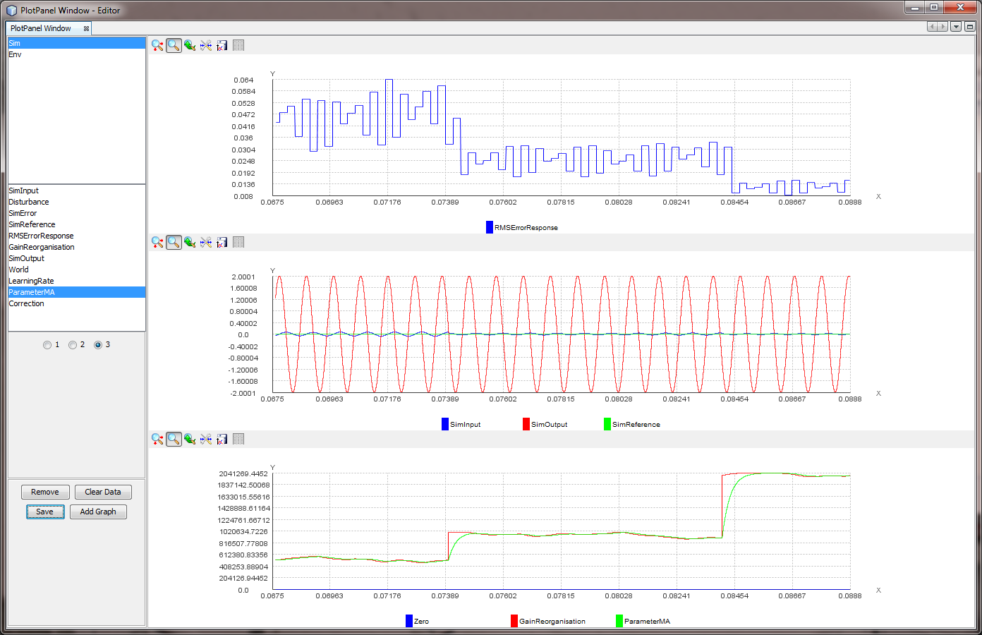
The objective is to minimize the RMS error
(or mean Absolute Error, which comes to the same thing), but you
need to ask about the “M” (Mean"). Over what period is it
averaged? You don’t want a boxcar average that takes the mean of
the last N values. You want a leaky integrator, just like the
leaky integrator in a control loop. Indeed, what you would be
building is exactly a control loop in which the perception is
the absolute or the squared error in the control loop whose
parameters you are changing.
The question, as in any control loop with a leaky integrator
output stage, is the balance between gain rate and leak rate.
The leak has to be slow enough to allow you to take account of
enough data, but not so slow that values from last week have
much influence on what you do in the next second or two. In your
case, I might suggest as a first cut that the leak rate of your
error-averaging integrator might be a few cycles of your sine
wave – say four or five at a guess.
How can the leak rate (which is the exponential moving average
smoothing factor) be set to the sine wave cycles (or number of
iterations)?
Re-reading my own comment, the leak rate in question is not that of
the control loop, but of the integrator that is part of the
calculation of the RMS error. My suspicion was that you might be
averaging over fixed time intervals rather than using a leaky
integrator. You just want to make the leak rate slow enough to avoid
getting mixed up with the phase of the sine wave and fast enough not
to get mixed up when the disturbance changes its character.
If you think of the problem as one of
building a control loop that has as its perception the control
quality of the loop whose parameters you are changing, and that
influences that perception by altering a parameter, I think you
will have better results.
Ok, another strategy for the plan.
Here's a possible functional diagram for a "reorganization control
loop" in which the loop shown deals with the magnitude of an e-coli
step, while a separate path (not shown) uses the derivative of the
QoC to set the probability of a tumble happening at each
computational iteration. That could also be inside the output
function (starred because it is not the same as the simple leaky
integrators of the perceptual control hierarchy even though it might
well include one).

If the intrinsic variable in question isn't QoC, it would not
normally be possible to assign its error value to any particular
control loop in the hierarchy. The same kind of reorganizing control
loop would apply, but interacting with a lot more control loops and
the parameters of their mutual interactions. That’s a whole 'nuther
discussion. I think it is part of the high-dimensional removal of
correlation by rotation discussion. But who knows?
Martin
···
http://www.mmtaylor.net/PCT/CSG2005/CSG2005bFittingData.ppt