[From Bruce Abbott (2015.02.05.2120 EST)]
Given the recent debate here about the behavior of passive equilibrium systems, I thought it would save a lot of “blah blah” argumentation to present a working simulation of such a system – in this case a mass-spring-damper system. I’ve created such a simulation (it’s a Windows App but should run on Macs that can spoof the Windows operating system) and posted it to my “Perceptual Control System Demos” Google website. If you would like a copy just follow this link (https://sites.google.com/site/perceptualcontroldemos/home/other-demos ) and click the “download” link under MassSpringDamperModel.zip. The zip file includes the executable (look for the .exe file extension in the Debug/Win32 subdirectory) and all necessary source code. You can copy the .exe file to your desktop or anywhere else you like as it does not require any other files to run. Then just double-click on the program’s icon.
The mass-spring-damper model is found in the Unit1.pas file, which is a text file so you can read it even if you don’t have the Delphi IDE. The model itself is contained in procedure TForm1.RunSim, as shown below:
procedure TForm1.RunSim;
// Computes the variables of the model each iteration
begin
Acc := (Force - dVel - sPos)/Mass; // net acceleration
Pos := Pos + (Vel + 0.5Accdt)*dt; // integrate position
Vel := Vel + Acc*dt; // integrate velocity
Time := Time + dt;
if Time >= ForceDur then Force := 0.0;
end;
The relevant variables and parameters are initialize in another procedure. During a model run, the RunSim procedure executes over and over in a loop, generating the behavioral dynamics of the system.
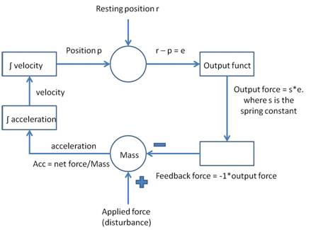
The first line computes the net acceleration due to forces acting on the mass: Force is an external force that compresses the spring; dVel gives the reaction force generated by the damper (d is the damping coefficient and Vel the velocity of the mass); sPos gives the reaction force generated by the spring, where s is the spring constant and Pos is the position of the mass (relative to its resting state, which is defined as zero. These forces are summed to give the net force and divided by the mass to give the acceleration of the mass as given by Newton’s force = Mass*Acc, solved for acceleration (i.e., Acc = force/mass).
The second line computes the new position from the previous one plus the change in position during the simulation time-step, dt. This change is found (approximately) by taking the previous velocity and adding one-half of the acceleration, multiplied by the time-step. The resulting new velocity is then multiplied by the time-step to yield the change in position.
The third line takes the old velocity and adds the change in velocity during the time-step, computed by multiplying the acceleration times the time-step.
The fourth line keeps track of the current time since the simulation began. This time is compared in the fifth line with the time stored in ForceDur (length of time the external force is allowed to continue acting on the mass); when the force has been acting for the allotted time, it is removed.
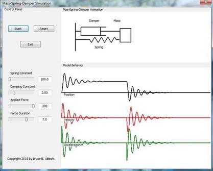
Here is a screen shot showing the simulation after it has been running long enough to complete the graphs shown in the bottom panel:
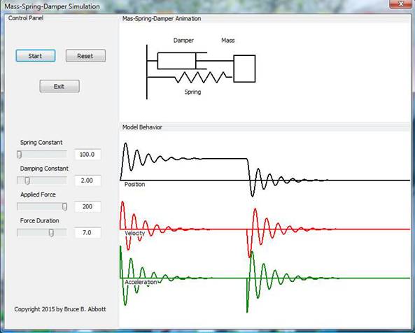
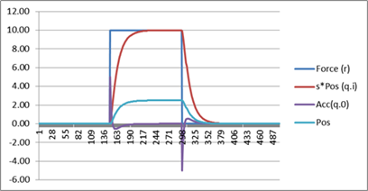
In this run, the external force pushed against the spring for seven seconds. The three graphs shown at bottom represent the position, velocity, and acceleration of the mass, respectively, over the course of several seconds. The sketch of the mass-spring-damper arrangement above the graphs shows action live.
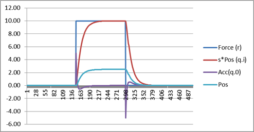
Note especially what happens to the position of the mass. At time zero the force is suddenly applied to the mass, accelerating it to the left, compressing the spring and moving the damper. In the graph, up indicates movement to the left. Initially there’s a bit of oscillation but this soon settles down to a new position well to the left of the resting position. This lays to rest any idea that the effect of the “negative feedback” is evident only after the external force is removed. If there were no “negative feedback, the impressed force would continue to accelerate the mass so long as the force persisted, but as you can see, this is not what happens. The system develops some degree of resistance to being disturbed from its resting state – enough resistance to bring the mass to a halt at a new position.
At the seven second mark the impressed force suddenly disappears, leaving the counterforces (“negative feedback”) to accelerate the mass toward the initial resting point. After some oscillation, the damping forces (which are proportional to velocity) convert the remaining energy of the system to heat and the system returns to its initial resting position.
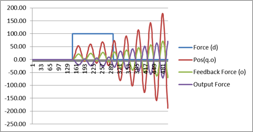
So here we have a system that resists disturbances (but does not resist them as strongly as a control system does) and returns to its initial equilibrium position once the disturbance is removed.
As the picture show, you can play around with various parameters (spring coefficient, damping coefficient, etc.) to see how they affect the way the system behaves. Be aware, however, that these parameters can be adjusted only while the simulation is not in the process of plotting the graphs. The system continues to run even after the graphs are complete, so you will need to press the “RESET” button before you can adjust the parameters. Then press the “START” button again to begin a new run with the altered parameters.