Omitted Variable Bias (was Re: Still Awaiting Rick's Reply)

Content-Type: application/vnd.ms-excel.sheet.macroEnabled.12;
  name="PowerLawRegressionwOVBCalculation.xlsm"
Content-Disposition: attachment;
  filename="PowerLawRegressionwOVBCalculation.xlsm"
X-Attachment-Id: f_is87heh40

Content-Type: application/pdf; name="2004_econometricssolutions.pdf"
Content-Disposition: attachment; filename="2004_econometricssolutions.pdf"
X-Attachment-Id: f_is87kqgd1

PowerLawRegressionwOVBCalculation.xlsm (614 KB)

2004_econometricssolutions.pdf (27.1 KB)

if pct is not phenomenological (in the sense that one can experience the claims it makes, and help the answer with that experience – like Powers’ exercices at the end of each chapter in BCP) then pct is not a good theory.Â

so, before you all continue to pretend you know maths by writing long emails, imagine yourself moving your finger on a surface following a curved line you draw and try to do it a different speeds and then at different accelerations across the curve and across trials.

then get rid of your your spreadshits and tell me what you see!

···

[From Rick Marken (2016.08.23.1830)]

Bruce Abbott (2016.08.23.1810 EDT)]

 Â

BA: As I have received no such reply after two days and you have during this same period posted several times on CSGnet, I assume that you have decided just to ignore my challenge. Perhaps I asked too much of you.

 RM: Actually, I did decide to ignore it. But while ignoring it I’ve made some discoveries that made it useful for me to un-ignore it.Â

Â

BA: Let’s make this simple. You have asserted as mathematical fact the following, based on an algebraic manipulation of the formula for the radius of curvature, R, in which you solve the equation for V:

Â

Rick Marken (2016.08.21.1620) –

Â

RM: This implies that you are thinking of curvature as a disturbance and velocity as the output that compensates for this disturbance. So you are, indeed, looking at the power law as an S-R (actually, a disturbance-output) relationship, with curvature (R) as the disturbance and velocity (V) Â as the output. The controlled variable would then be some function of curvature and velocity (CV = f( R, V). Â The problem is that, for this to be true, R and V must have independent effects on the CV. And they can’t because the value of R depends completely on the value of V and vice versa.

Â

BA: I take this statement to constitute a prediction based on your belief that the equation for R implies that V and R, as observed in the data, cannot have independent effects; rather, V must always be a function of R to the one-third power (more or less; you leave yourself a bit of wiggle room by hypothesizing that leaving D out of the regression permits some of the relationship to be observed into the error term). Therefore, if a data set can be found in which V and R do not vary as you predict, this would constitute a firm refutation of your statement.

RM: My statement above, that you highlighted in red, is not a model of clarity. So let me start over:Â

RM: I claim that the relationship between measures of R and V, for any curved movement trajectory, is given by:

V = Â D1/3Â *R1/3Â Â Â Â Â Â Â Â Â Â Â Â Â Â Â Â Â Â Â Â Â Â Â Â Â Â

Â

where D is |dXd2Y-d2XdY|. Different movement trajectories will result in different patterns of variation in these three variables. If you look at the relationship between just V and R for different movement trajectories, the form of that relationship will be different for each one. The relationship between V and R can be perfectly linear (as Bruce has shown) or it can be approximately linear or it can be a power function with a coefficient of 1/3 or a power function with a coefficient that is very different from 1/3 or whatever.  But the equation above says that the true relationship between R and V is a power function with a coefficient of 1/3. This will only be seen, however, if the variable D is included in an analysis that is aimed at evaluating the form of the relationship between R and V.

RM: Power law researchers evaluate the form of the relationship between R and V using regression analysis. The goal of the analysis is to determine whether or not a movement trajectory conforms to the “power law” – the “law” being that the power coefficient relating R to V is 1/3. They do this by regressing log(R) on log(V), which assumes that there is a power function relationship between R and V. They often find that a power function fits the data well (in terms of R^2) often with a power coefficient close to 1/3 (hence the idea that it’s a “law”. But they also get different estimates of the power coefficient; sometimes the estimate is nowhere near 1/3; and sometimes the R^2 fit of a power function to the data is very small. I presume that these are considered to be cases – when the power coefficient is not 1/3 and/or R^2 is not close to .9 –  where the movement trajectory fails to conform to the power law.

RM: My analysis says that all these differences in the results you get from using regression analyses to determine the power law are a result of regressing log(R) on log(V) leaving out log (D). The proper regression equation to use to account for the variance in log (V) is:

log (V) = a + b1log(R) + b2 log (D)

RM: When this regression equation is used to evaluate the power coefficient for log (R) it  is always found to be the  true value, 1/3, and the  R^2 for the regression is always found to be 1.0.Â

RM: But power law researchers evaluate the power law using a regression equation that leaves out log (D) as follows:Â

log (V) = a + b1*log(R)

RM: The result is that they find values for the power coefficient, b1, that differ somewhat (and occasionally a lot) from 1/3 for different movement trajectories. I’ve argued that this is a statistical artifact, the value of b1 that is found by the regression without log(D) as a predictor being “biased” away from the true value of b1 (call it b1’) because of variance in log(V) associated with the variance in the omitted variable, log(D).Â

RM: I assumed that the variance contributed to log(V) would be different for different movement trajectories and that this would account for the difference in the estimates of the “power law” coefficient (b1) that are obtained when only log(R) and log(V) are included in the regressions. This remained no more than an assumption until today when I learned that it is possible to determine the exact amount by which  the regression coefficient  is “biased” away from it’s true value when another important explanatory variable is left out of the analysis. The way it’s done is by using something called “Omitted Variables Bias” analysis or OVB.Â

RM: OVB analysis lets you calculate exactly how much an observed regression coefficient will deviate from its true value when another variable is omitted from the analysis. The OVB calculation looks like this:

 b1 = b1’ + [b2’ * (Cov(log(R),log(D))/Var(log(R))]Â

RM: In the case of the power law studies, b1 is the observed value of the coefficient of log(R) when regressing log(R) on log(V), b1’ is the true value of this coefficient, and b2’ is the true value of the coefficient of the of the omitted variable, log(D). Since we typically don’t know the true values of b1 and b2, OVB analysis is mainly used to estimate how biased (and in what direction) your estimate of b1’ might be as a result of omitting a variable. The bias is measured by [b2’ * (Cov(R,D)/Var(R)].  But in the case of the power law, we know, from my equation V =  D1/3 *R1/3, that the true value of b1, b1’, is 1/3 and the true value of b2, b2’, is 1/3. So we can use the OVB equation above to predict exactly what the observed power law coefficient, b1, will be in a power law analysis for any movement trajectory that leaves out the variable log(D) from the analysis. The OVB equation is:

 b1 = 1/3 + [1/3* (Cov(log(R),log(D))/Var(log(R))] Â

RM: I’m attaching a spreadsheet to show how nicely this works. I’ve simplified the spreadsheet so that you can either collect data from your own movements or from randomly generated squiggle movements. When you collect data just move the cursor around the screen any way you want. There is no tracking; just moving. Move the cursor fast through curves and slow on straightaways if you like. Make any kind of crazy movement you like. When done, press the “Analyze Human Input” button and see the results of the  power law analyses of the movement.Â

RM: The relevant analyses are the one at the top (log(R) on log(V)) and second from the bottom (log(C) on log (A)). Next to the power coefficients that are obtained from these analyses I have computed the value of the power coefficient (“Expected beta”, corresponding to b1 in the OVB equation) that is expected when the variable log (D) is left out of the analysis, as it is in these two analyses.Â

RM: Note that the expected value of beta, based on OVB analysis, is exactly the same as the observed value of beta. I think this proves beyond a reasonable doubt that the power coefficient observed in studies of movement is a statistical artifact; a side effect of leaving log (D) out of the regression analyses used to find the power law. The power law clearly has nothing to do with how the movement is produced; the explanation of how the movement is produced is already at hand; it’s called PCT.

RM: Happy moving.Â

Best regards

Rick

PS. I’m also attaching a little writeup on OVB analysis, produced by “normal” scientists – at Harvard yet! The relevant material is in Econometrics Question # 2.Â


Richard S. MarkenÂ

“The childhood of the human race is far from over. We
have a long way to go before most people will understand that what they do for
others is just as important to their well-being as what they do for
themselves.” – William T. Powers

When I do Rick’s I never get the power law relationship of .33 or .67 but I do when it includes D in the equation. But this isn’t the equation that the power law researchers use. So I might need explaining again!
When I do Alex’s I find that I overshoot the curve (curve less than intended) when I try to negotiate a curve fast. This happens to my car too and I thought it was due to centripetal force but maybe I am wrong…

Warren

···

On Wed, Aug 24, 2016 at 7:50 AM, Alex Gomez-Marin agomezmarin@gmail.com wrote:

if pct is not phenomenological (in the sense that one can experience the claims it makes, and help the answer with that experience – like Powers’ exercices at the end of each chapter in BCP) then pct is not a good theory.Â

so, before you all continue to pretend you know maths by writing long emails, imagine yourself moving your finger on a surface following a curved line you draw and try to do it a different speeds and then at different accelerations across the curve and across trials.

then get rid of your your spreadshits and tell me what you see!

On Wednesday, 24 August 2016, Richard Marken rsmarken@gmail.com wrote:

[From Rick Marken (2016.08.23.1830)]

Bruce Abbott (2016.08.23.1810 EDT)]

 Â

BA: As I have received no such reply after two days and you have during this same period posted several times on CSGnet, I assume that you have decided just to ignore my challenge. Perhaps I asked too much of you.

 RM: Actually, I did decide to ignore it. But while ignoring it I’ve made some discoveries that made it useful for me to un-ignore it.Â

Â

BA: Let’s make this simple. You have asserted as mathematical fact the following, based on an algebraic manipulation of the formula for the radius of curvature, R, in which you solve the equation for V:

Â

Rick Marken (2016.08.21.1620) –

RM: This implies that you are thinking of curvature as a disturbance and velocity as the output that compensates for this disturbance. So you are, indeed, looking at the power law as an S-R (actually, a disturbance-output) relationship, with curvature (R) as the disturbance and velocity (V) Â as the output. The controlled variable would then be some function of curvature and velocity (CV = f( R, V). Â The problem is that, for this to be true, R and V must have independent effects on the CV. And they can’t because the value of R depends completely on the value of V and vice versa.

Â

BA: I take this statement to constitute a prediction based on your belief that the equation for R implies that V and R, as observed in the data, cannot have independent effects; rather, V must always be a function of R to the one-third power (more or less; you leave yourself a bit of wiggle room by hypothesizing that leaving D out of the regression permits some of the relationship to be observed into the error term). Therefore, if a data set can be found in which V and R do not vary as you predict, this would constitute a firm refutation of your statement.

RM: My statement above, that you highlighted in red, is not a model of clarity. So let me start over:Â

RM: I claim that the relationship between measures of R and V, for any curved movement trajectory, is given by:

V = Â D1/3Â *R1/3Â Â Â Â Â Â Â Â Â Â Â Â Â Â Â Â Â Â Â Â Â Â Â Â Â Â

Â

where D is |dXd2Y-d2XdY|. Different movement trajectories will result in different patterns of variation in these three variables. If you look at the relationship between just V and R for different movement trajectories, the form of that relationship will be different for each one. The relationship between V and R can be perfectly linear (as Bruce has shown) or it can be approximately linear or it can be a power function with a coefficient of 1/3 or a power function with a coefficient that is very different from 1/3 or whatever.  But the equation above says that the true relationship between R and V is a power function with a coefficient of 1/3. This will only be seen, however, if the variable D is included in an analysis that is aimed at evaluating the form of the relationship between R and V.

RM: Power law researchers evaluate the form of the relationship between R and V using regression analysis. The goal of the analysis is to determine whether or not a movement trajectory conforms to the “power law” – the “law” being that the power coefficient relating R to V is 1/3. They do this by regressing log(R) on log(V), which assumes that there is a power function relationship between R and V. They often find that a power function fits the data well (in terms of R^2) often with a power coefficient close to 1/3 (hence the idea that it’s a “law”. But they also get different estimates of the power coefficient; sometimes the estimate is nowhere near 1/3; and sometimes the R^2 fit of a power function to the data is very small. I presume that these are considered to be cases – when the power coefficient is not 1/3 and/or R^2 is not close to .9 –  where the movement trajectory fails to conform to the power law.

RM: My analysis says that all these differences in the results you get from using regression analyses to determine the power law are a result of regressing log(R) on log(V) leaving out log (D). The proper regression equation to use to account for the variance in log (V) is:

log (V) = a + b1log(R) + b2 log (D)

RM: When this regression equation is used to evaluate the power coefficient for log (R) it  is always found to be the  true value, 1/3, and the  R^2 for the regression is always found to be 1.0.Â

RM: But power law researchers evaluate the power law using a regression equation that leaves out log (D) as follows:Â

log (V) = a + b1*log(R)

RM: The result is that they find values for the power coefficient, b1, that differ somewhat (and occasionally a lot) from 1/3 for different movement trajectories. I’ve argued that this is a statistical artifact, the value of b1 that is found by the regression without log(D) as a predictor being “biased” away from the true value of b1 (call it b1’) because of variance in log(V) associated with the variance in the omitted variable, log(D).Â

RM: I assumed that the variance contributed to log(V) would be different for different movement trajectories and that this would account for the difference in the estimates of the “power law” coefficient (b1) that are obtained when only log(R) and log(V) are included in the regressions. This remained no more than an assumption until today when I learned that it is possible to determine the exact amount by which  the regression coefficient  is “biased” away from it’s true value when another important explanatory variable is left out of the analysis. The way it’s done is by using something called “Omitted Variables Bias” analysis or OVB.Â

RM: OVB analysis lets you calculate exactly how much an observed regression coefficient will deviate from its true value when another variable is omitted from the analysis. The OVB calculation looks like this:

 b1 = b1’ + [b2’ * (Cov(log(R),log(D))/Var(log(R))]Â

RM: In the case of the power law studies, b1 is the observed value of the coefficient of log(R) when regressing log(R) on log(V), b1’ is the true value of this coefficient, and b2’ is the true value of the coefficient of the of the omitted variable, log(D). Since we typically don’t know the true values of b1 and b2, OVB analysis is mainly used to estimate how biased (and in what direction) your estimate of b1’ might be as a result of omitting a variable. The bias is measured by [b2’ * (Cov(R,D)/Var(R)].  But in the case of the power law, we know, from my equation V =  D1/3 *R1/3, that the true value of b1, b1’, is 1/3 and the true value of b2, b2’, is 1/3. So we can use the OVB equation above to predict exactly what the observed power law coefficient, b1, will be in a power law analysis for any movement trajectory that leaves out the variable log(D) from the analysis. The OVB equation is:

 b1 = 1/3 + [1/3* (Cov(log(R),log(D))/Var(log(R))] Â

RM: I’m attaching a spreadsheet to show how nicely this works. I’ve simplified the spreadsheet so that you can either collect data from your own movements or from randomly generated squiggle movements. When you collect data just move the cursor around the screen any way you want. There is no tracking; just moving. Move the cursor fast through curves and slow on straightaways if you like. Make any kind of crazy movement you like. When done, press the “Analyze Human Input” button and see the results of the  power law analyses of the movement.Â

RM: The relevant analyses are the one at the top (log(R) on log(V)) and second from the bottom (log(C) on log (A)). Next to the power coefficients that are obtained from these analyses I have computed the value of the power coefficient (“Expected beta”, corresponding to b1 in the OVB equation) that is expected when the variable log (D) is left out of the analysis, as it is in these two analyses.Â

RM: Note that the expected value of beta, based on OVB analysis, is exactly the same as the observed value of beta. I think this proves beyond a reasonable doubt that the power coefficient observed in studies of movement is a statistical artifact; a side effect of leaving log (D) out of the regression analyses used to find the power law. The power law clearly has nothing to do with how the movement is produced; the explanation of how the movement is produced is already at hand; it’s called PCT.

RM: Happy moving.Â

Best regards

Rick

PS. I’m also attaching a little writeup on OVB analysis, produced by “normal” scientists – at Harvard yet! The relevant material is in Econometrics Question # 2.Â


Richard S. MarkenÂ

“The childhood of the human race is far from over. We
have a long way to go before most people will understand that what they do for
others is just as important to their well-being as what they do for
themselves.” – William T. Powers

Dr Warren Mansell
Reader in Clinical Psychology

School of Health Sciences
2nd Floor Zochonis Building
University of Manchester
Oxford Road
Manchester M13 9PL
Email: warren.mansell@manchester.ac.uk
Â
Tel: +44 (0) 161 275 8589
Â
Website: http://www.psych-sci.manchester.ac.uk/staff/131406
Â
Advanced notice of a new transdiagnostic therapy manual, authored by Carey, Mansell & Tai - Principles-Based Counselling and Psychotherapy: A Method of Levels Approach

Available Now

Check www.pctweb.org for further information on Perceptual Control Theory

[From Fred Nickols (2016.08.24.0635 ET)]

I might not be able to do fancy math but I think I can follow simple instructions. First, I drew a curve, an arc about 4.5 inches across the bottom and 1.5 inches high (if it were vertical).

Then I tried following the line with the forefinger of my right hand. I did this at various fast and slow speeds. I also did it accelerating at various rates.

I was able to follow the line with my forefinger. Although I varied speed and rate of acceleration, I suspect that I did not move at any speed or rate of acceleration that would cause me to not be able to track the curve.

So?

Fred Nickols

···

From: Alex Gomez-Marin [mailto:agomezmarin@gmail.com]
Sent: Wednesday, August 24, 2016 2:51 AM
To: csgnet@lists.illinois.edu
Subject: Re: Omitted Variable Bias (was Re: Still Awaiting Rick’s Reply)

if pct is not phenomenological (in the sense that one can experience the claims it makes, and help the answer with that experience – like Powers’ exercices at the end of each chapter in BCP) then pct is not a good theory.

so, before you all continue to pretend you know maths by writing long emails, imagine yourself moving your finger on a surface following a curved line you draw and try to do it a different speeds and then at different accelerations across the curve and across trials.

then get rid of your your spreadshits and tell me what you see!

On Wednesday, 24 August 2016, Richard Marken rsmarken@gmail.com wrote:

[From Rick Marken (2016.08.23.1830)]

Bruce Abbott (2016.08.23.1810 EDT)]

BA: As I have received no such reply after two days and you have during this same period posted several times on CSGnet, I assume that you have decided just to ignore my challenge. Perhaps I asked too much of you.

RM: Actually, I did decide to ignore it. But while ignoring it I’ve made some discoveries that made it useful for me to un-ignore it.

BA: Let’s make this simple. You have asserted as mathematical fact the following, based on an algebraic manipulation of the formula for the radius of curvature, R, in which you solve the equation for V:

Rick Marken (2016.08.21.1620) –

RM: This implies that you are thinking of curvature as a disturbance and velocity as the output that compensates for this disturbance. So you are, indeed, looking at the power law as an S-R (actually, a disturbance-output) relationship, with curvature (R) as the disturbance and velocity (V) as the output. The controlled variable would then be some function of curvature and velocity (CV = f( R, V). The problem is that, for this to be true, R and V must have independent effects on the CV. And they can’t because the value of R depends completely on the value of V and vice versa.

BA: I take this statement to constitute a prediction based on your belief that the equation for R implies that V and R, as observed in the data, cannot have independent effects; rather, V must always be a function of R to the one-third power (more or less; you leave yourself a bit of wiggle room by hypothesizing that leaving D out of the regression permits some of the relationship to be observed into the error term). Therefore, if a data set can be found in which V and R do not vary as you predict, this would constitute a firm refutation of your statement.

RM: My statement above, that you highlighted in red, is not a model of clarity. So let me start over:

RM: I claim that the relationship between measures of R and V, for any curved movement trajectory, is given by:

V = D1/3 *R1/3

where D is |dXd2Y-d2XdY|. Different movement trajectories will result in different patterns of variation in these three variables. If you look at the relationship between just V and R for different movement trajectories, the form of that relationship will be different for each one. The relationship between V and R can be perfectly linear (as Bruce has shown) or it can be approximately linear or it can be a power function with a coefficient of 1/3 or a power function with a coefficient that is very different from 1/3 or whatever. But the equation above says that the true relationship between R and V is a power function with a coefficient of 1/3. This will only be seen, however, if the variable D is included in an analysis that is aimed at evaluating the form of the relationship between R and V.

RM: Power law researchers evaluate the form of the relationship between R and V using regression analysis. The goal of the analysis is to determine whether or not a movement trajectory conforms to the “power law” – the “law” being that the power coefficient relating R to V is 1/3. They do this by regressing log(R) on log(V), which assumes that there is a power function relationship between R and V. They often find that a power function fits the data well (in terms of R^2) often with a power coefficient close to 1/3 (hence the idea that it’s a “law”. But they also get different estimates of the power coefficient; sometimes the estimate is nowhere near 1/3; and sometimes the R^2 fit of a power function to the data is very small. I presume that these are considered to be cases – when the power coefficient is not 1/3 and/or R^2 is not close to .9 – where the movement trajectory fails to conform to the power law.

RM: My analysis says that all these differences in the results you get from using regression analyses to determine the power law are a result of regressing log(R) on log(V) leaving out log (D). The proper regression equation to use to account for the variance in log (V) is:

log (V) = a + b1log(R) + b2 log (D)

RM: When this regression equation is used to evaluate the power coefficient for log (R) it is always found to be the true value, 1/3, and the R^2 for the regression is always found to be 1.0.

RM: But power law researchers evaluate the power law using a regression equation that leaves out log (D) as follows:

log (V) = a + b1*log(R)

RM: The result is that they find values for the power coefficient, b1, that differ somewhat (and occasionally a lot) from 1/3 for different movement trajectories. I’ve argued that this is a statistical artifact, the value of b1 that is found by the regression without log(D) as a predictor being “biased” away from the true value of b1 (call it b1’) because of variance in log(V) associated with the variance in the omitted variable, log(D).

RM: I assumed that the variance contributed to log(V) would be different for different movement trajectories and that this would account for the difference in the estimates of the “power law” coefficient (b1) that are obtained when only log(R) and log(V) are included in the regressions. This remained no more than an assumption until today when I learned that it is possible to determine the exact amount by which the regression coefficient is “biased” away from it’s true value when another important explanatory variable is left out of the analysis. The way it’s done is by using something called “Omitted Variables Bias” analysis or OVB.

RM: OVB analysis lets you calculate exactly how much an observed regression coefficient will deviate from its true value when another variable is omitted from the analysis. The OVB calculation looks like this:

b1 = b1’ + [b2’ * (Cov(log(R),log(D))/Var(log(R))]

RM: In the case of the power law studies, b1 is the observed value of the coefficient of log(R) when regressing log(R) on log(V), b1’ is the true value of this coefficient, and b2’ is the true value of the coefficient of the of the omitted variable, log(D). Since we typically don’t know the true values of b1 and b2, OVB analysis is mainly used to estimate how biased (and in what direction) your estimate of b1’ might be as a result of omitting a variable. The bias is measured by [b2’ * (Cov(R,D)/Var(R)]. But in the case of the power law, we know, from my equation V = D1/3 *R1/3, that the true value of b1, b1’, is 1/3 and the true value of b2, b2’, is 1/3. So we can use the OVB equation above to predict exactly what the observed power law coefficient, b1, will be in a power law analysis for any movement trajectory that leaves out the variable log(D) from the analysis. The OVB equation is:

b1 = 1/3 + [1/3* (Cov(log(R),log(D))/Var(log(R))]

RM: I’m attaching a spreadsheet to show how nicely this works. I’ve simplified the spreadsheet so that you can either collect data from your own movements or from randomly generated squiggle movements. When you collect data just move the cursor around the screen any way you want. There is no tracking; just moving. Move the cursor fast through curves and slow on straightaways if you like. Make any kind of crazy movement you like. When done, press the “Analyze Human Input” button and see the results of the power law analyses of the movement.

RM: The relevant analyses are the one at the top (log(R) on log(V)) and second from the bottom (log(C) on log (A)). Next to the power coefficients that are obtained from these analyses I have computed the value of the power coefficient (“Expected beta”, corresponding to b1 in the OVB equation) that is expected when the variable log (D) is left out of the analysis, as it is in these two analyses.

RM: Note that the expected value of beta, based on OVB analysis, is exactly the same as the observed value of beta. I think this proves beyond a reasonable doubt that the power coefficient observed in studies of movement is a statistical artifact; a side effect of leaving log (D) out of the regression analyses used to find the power law. The power law clearly has nothing to do with how the movement is produced; the explanation of how the movement is produced is already at hand; it’s called PCT.

RM: Happy moving.

Best regards

Rick

PS. I’m also attaching a little writeup on OVB analysis, produced by “normal” scientists – at Harvard yet! The relevant material is in Econometrics Question # 2.

Richard S. Marken

“The childhood of the human race is far from over. We have a long way to go before most people will understand that what they do for others is just as important to their well-being as what they do for themselves.” – William T. Powers

RM : The power law clearly has nothing to do with how the movement is produced; the explanation of how the movement is produced is already at hand; it’s called PCT.

HB : It seems to me that you »went up a level« or maybe two J All you have to do now is to understand PCT right.

RM: I don’t think this is what defines a good theory. Phenomenology can be quite misleading. Indeed, it was misleading phenomenology that convinced me that PCT was the right approach to understanding behavior. The misleading phenomenology occurs in the tracking task that Powers used to illustrate the basic facts of control. An example of this tracking task is at http://www.mindreadings.com/ControlDemo/BasicTrack.html.

HB : You started again. It seems that you didn’t go »down level or two«, but that you exit perceptual hierarchy. You are talking about control in organisms environment.

When will you stop pushing your demos into »first plan« of PCT. This is forum for Bill’s PCT if you didn’t noticed. Your demos are mostly wrong so they don’t represent right PCT. You are showing just partly the main principle that could be involved in PCT explanation of behavior. Aligning two »vertical lines« does not control the behavior or perception or whatever. Neither »Control of behavior« align two lines. The »controlled variable« (distance between curzor and target) is not what is controlled. How can control come from outside through input of the system and »control« behavior (output). Behavior is never controlled from outside. It’s always effected from inside where references are formed.

You started again with your RCT. How can input contain control from outside ? When will you learn Rick that this is not what PCT is about ??? Why don’t you read article of Henry Yin again ???

RM: The phenomenology of this task for most people is that they are moving the mouse in the opposite direction as the cursor in order to keep the cursor on target: It feels like you move the mouse right when the cursor moves to the left of the target and to the left when the cursor moves to the right of the target.

HB : I’m pushing mouse in all directions when trying to aline two »vertical lines«. Sometimes I have to push in the same direction the line is moving, and sometimes in opposite direction. My computer doesn’t work well ??? Or your demo is wrong ???

RM: Of course, the PCT model accounts for the behavior in the tracking task perfectly (as see in the demo).

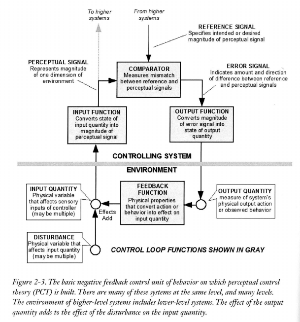
HB : You can dream of it. It’s far from working perfectly and even if it does it says nothing about perceptual control in hierarchy, because there can be no »controled variable« in outer environment and of course no »behavior control«. See Bill’s diagram…. In his books you will also find explanation why your demo is wrongly showing »Perceptual Control«. Just start reading his literature and you’ll have right »phenomenology« in your head.

RM : And the model also explains why the phenomenology is misleading.

HB : Your RCT with your wrong demo is misleading…. And your confuseed imagination (phenomenology)…

RM : It’s because the cursor movement is an input and an output at the same time.

HB :

We already established that »contol« events doesn’t happen at the same time. It’s again you imagination (phenomenology). There is always some time delay between perceiving certain position and »reacting« on that »certain position«, because events in nervous system are not so fast. This can be traced in nervous system activity. Afferent neuron (input) and efferent neuron (outpout) never fire at the same time, but they could be very close if control is happening fast. But we have already talked about it.

HB earlier : Every physiologist knows and could explain to you that El Hady was right : whatever is happening in control loop is sequence of »cause-effect« events through the loop (some time delays).

RM earlier : You are absolutely right.

HB So it’s probably the events that happen quite fast those who made your wrong conclussions. Your »phenomenalistic« brains doesn’t recognise the difference and you seem to see that everything on this world is happening at the same time.

And I’m wondering when you’ll stop »stupiding« people arround with your riddicoulus (behavioristic) demos and your RCT, where behavior is control, and there is some »control variable« in outer environment, and everything is happening at the same time. What do you want ??? That public start laughing to PCT ??? Show me in Bill’s diagram (LCS III) where you see all this things happening ???

Best,

Boris

···

From: Richard Marken [mailto:rsmarken@gmail.com]
Sent: Wednesday, August 24, 2016 3:33 AM
To: csgnet@lists.illinois.edu
Cc: Henry Yin; Richard Marken
Subject: Omitted Variable Bias (was Re: Still Awaiting Rick’s Reply)

[From Rick Marken (2016.08.23.1830)]

Bruce Abbott (2016.08.23.1810 EDT)]

BA: As I have received no such reply after two days and you have during this same period posted several times on CSGnet, I assume that you have decided just to ignore my challenge. Perhaps I asked too much of you.

RM: Actually, I did decide to ignore it. But while ignoring it I’ve made some discoveries that made it useful for me to un-ignore it.

BA: Let’s make this simple. You have asserted as mathematical fact the following, based on an algebraic manipulation of the formula for the radius of curvature, R, in which you solve the equation for V:

Rick Marken (2016.08.21.1620) –

RM: This implies that you are thinking of curvature as a disturbance and velocity as the output that compensates for this disturbance. So you are, indeed, looking at the power law as an S-R (actually, a disturbance-output) relationship, with curvature (R) as the disturbance and velocity (V) as the output. The controlled variable would then be some function of curvature and velocity (CV = f( R, V). The problem is that, for this to be true, R and V must have independent effects on the CV. And they can’t because the value of R depends completely on the value of V and vice versa.

BA: I take this statement to constitute a prediction based on your belief that the equation for R implies that V and R, as observed in the data, cannot have independent effects; rather, V must always be a function of R to the one-third power (more or less; you leave yourself a bit of wiggle room by hypothesizing that leaving D out of the regression permits some of the relationship to be observed into the error term). Therefore, if a data set can be found in which V and R do not vary as you predict, this would constitute a firm refutation of your statement.

RM: My statement above, that you highlighted in red, is not a model of clarity. So let me start over:

RM: I claim that the relationship between measures of R and V, for any curved movement trajectory, is given by:

V = D1/3 *R1/3

where D is |dXd2Y-d2XdY|. Different movement trajectories will result in different patterns of variation in these three variables. If you look at the relationship between just V and R for different movement trajectories, the form of that relationship will be different for each one. The relationship between V and R can be perfectly linear (as Bruce has shown) or it can be approximately linear or it can be a power function with a coefficient of 1/3 or a power function with a coefficient that is very different from 1/3 or whatever. But the equation above says that the true relationship between R and V is a power function with a coefficient of 1/3. This will only be seen, however, if the variable D is included in an analysis that is aimed at evaluating the form of the relationship between R and V.

RM: Power law researchers evaluate the form of the relationship between R and V using regression analysis. The goal of the analysis is to determine whether or not a movement trajectory conforms to the “power law” – the “law” being that the power coefficient relating R to V is 1/3. They do this by regressing log(R) on log(V), which assumes that there is a power function relationship between R and V. They often find that a power function fits the data well (in terms of R^2) often with a power coefficient close to 1/3 (hence the idea that it’s a “law”. But they also get different estimates of the power coefficient; sometimes the estimate is nowhere near 1/3; and sometimes the R^2 fit of a power function to the data is very small. I presume that these are considered to be cases – when the power coefficient is not 1/3 and/or R^2 is not close to .9 – where the movement trajectory fails to conform to the power law.

RM: My analysis says that all these differences in the results you get from using regression analyses to determine the power law are a result of regressing log(R) on log(V) leaving out log (D). The proper regression equation to use to account for the variance in log (V) is:

log (V) = a + b1log(R) + b2 log (D)

RM: When this regression equation is used to evaluate the power coefficient for log (R) it is always found to be the true value, 1/3, and the R^2 for the regression is always found to be 1.0.

RM: But power law researchers evaluate the power law using a regression equation that leaves out log (D) as follows:

log (V) = a + b1*log(R)

RM: The result is that they find values for the power coefficient, b1, that differ somewhat (and occasionally a lot) from 1/3 for different movement trajectories. I’ve argued that this is a statistical artifact, the value of b1 that is found by the regression without log(D) as a predictor being “biased” away from the true value of b1 (call it b1’) because of variance in log(V) associated with the variance in the omitted variable, log(D).

RM: I assumed that the variance contributed to log(V) would be different for different movement trajectories and that this would account for the difference in the estimates of the “power law” coefficient (b1) that are obtained when only log(R) and log(V) are included in the regressions. This remained no more than an assumption until today when I learned that it is possible to determine the exact amount by which the regression coefficient is “biased” away from it’s true value when another important explanatory variable is left out of the analysis. The way it’s done is by using something called “Omitted Variables Bias” analysis or OVB.

RM: OVB analysis lets you calculate exactly how much an observed regression coefficient will deviate from its true value when another variable is omitted from the analysis. The OVB calculation looks like this:

b1 = b1’ + [b2’ * (Cov(log(R),log(D))/Var(log(R))]

RM: In the case of the power law studies, b1 is the observed value of the coefficient of log(R) when regressing log(R) on log(V), b1’ is the true value of this coefficient, and b2’ is the true value of the coefficient of the of the omitted variable, log(D). Since we typically don’t know the true values of b1 and b2, OVB analysis is mainly used to estimate how biased (and in what direction) your estimate of b1’ might be as a result of omitting a variable. The bias is measured by [b2’ * (Cov(R,D)/Var(R)]. But in the case of the power law, we know, from my equation V = D1/3 *R1/3, that the true value of b1, b1’, is 1/3 and the true value of b2, b2’, is 1/3. So we can use the OVB equation above to predict exactly what the observed power law coefficient, b1, will be in a power law analysis for any movement trajectory that leaves out the variable log(D) from the analysis. The OVB equation is:

b1 = 1/3 + [1/3* (Cov(log(R),log(D))/Var(log(R))]

RM: I’m attaching a spreadsheet to show how nicely this works. I’ve simplified the spreadsheet so that you can either collect data from your own movements or from randomly generated squiggle movements. When you collect data just move the cursor around the screen any way you want. There is no tracking; just moving. Move the cursor fast through curves and slow on straightaways if you like. Make any kind of crazy movement you like. When done, press the “Analyze Human Input” button and see the results of the power law analyses of the movement.

RM: The relevant analyses are the one at the top (log(R) on log(V)) and second from the bottom (log(C) on log (A)). Next to the power coefficients that are obtained from these analyses I have computed the value of the power coefficient (“Expected beta”, corresponding to b1 in the OVB equation) that is expected when the variable log (D) is left out of the analysis, as it is in these two analyses.

RM: Note that the expected value of beta, based on OVB analysis, is exactly the same as the observed value of beta. I think this proves beyond a reasonable doubt that the power coefficient observed in studies of movement is a statistical artifact; a side effect of leaving log (D) out of the regression analyses used to find the power law. The power law clearly has nothing to do with how the movement is produced; the explanation of how the movement is produced is already at hand; it’s called PCT.

RM: Happy moving.

Best regards

Rick

PS. I’m also attaching a little writeup on OVB analysis, produced by “normal” scientists – at Harvard yet! The relevant material is in Econometrics Question # 2.

Richard S. Marken

“The childhood of the human race is far from over. We have a long way to go before most people will understand that what they do for others is just as important to their well-being as what they do for themselves.” – William T. Powers