[Martin Taylor
2008.12.18.15.32]
[From Bill Powers
(2008.12.18.1029 MST)]
Martin Taylor 2008.12.18.11.09 –
You can’t really talk about a
signal-to-noise ratio based on the plots in this paper (
http://www.biolbull.org/cgi/reprint/199/2/176.pdf ). The plot is of
time from one impulse to the next, and nothing happens at all in between
pulses.
Actually, the y-axis in that paper has units of impulses per second, the
reciprocal of inter-impulse time.
The y-axis does, but the plot doesn’t, nor does the methodology.
I have no idea what you mean by that.
The axis shows the inverse of
the inter-pulse interval for each impulse, so far as I understand
it.
Yes, and that has units of frequency – 1/time, or sec^-1, a standard way
of writing “per second.” An impulse rate of 20 per second is
equivalent to an impulse interval of 1/20 second.
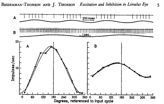
The same is true of the
Beiderman-Thorson and Thorson paper: The blips are closest together at
the highest light intensity, and the line plots are shown with the Y-axis
labeled “impulses/sec.”
Yes. The Thorsons averaged over
long periods. You have to cut them some slack on this, since they
published in 1971, and almost certainly did not have a pulse-by-pulse
record in their computer to analyze.
They probably used a strip-chart recorder or photographed an
oscilloscope, or used an A/D converter storing data into a computer. I
used all those tools long before 1971. How long ago do you think 1971
was? I used Tektronix oscilloscopes throughout the 1960s and 1970s as
well as desktop minicomputers (A Dec PDP8-s and later a Data General
Nova).
But there is actually one place
in the paper (which I have now read more carefully) where they suggest a
measure of variability that might be used. They say SD at 4.5
impulses/sec is about 0.1 impulse/sec,
No, they say “for example, SD of
interval/mean interval = 0.1 at 4.5
spikes per sec)”. The mean pulse rate was 4.5 spikes
per second and the ratio (SD of interval)/(mean interval) was 0.1,
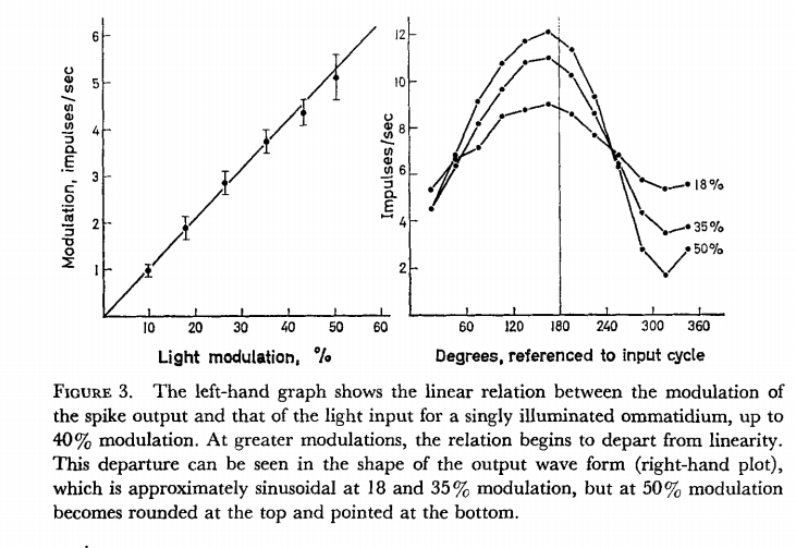
meaning that one standard deviation was 0.45 pulses per second. You can
see this in Fig 3:
In the left-hand graph you can see the error bars indicating the standard
deviations (I presume) at each degree of modulation. On the right are
indicated the variations in signal (in impulses/sec) as the illumination
goes through its cycle. Clearly, the standard deviation represents a mean
departure of the signal amplitude from the light intensity at each point
during the cycle. The signal-to-noise ratio is about 10:1, assuming it’s
the same at all illumination levels.
David Goldstein and I were
talking about this yesterday. Certainly the neural signals traveling in
axons are a train of impulses. Why don’t we perceive them that way? What
we perceive instead is a smoothly-varying intensity, or at least an
intensity that varies in steps too small to notice. It would seem that
the correlate of conscious perception that best fits experience is not
the train of impulses, but the concentrations of messenger chemicals
inside the neuron’s cell-body. The time-constant of changes in chemical
concentration as well as the electrical capacitance of the cell wall see
to it that the necessary smoothing occurs.
That’s an interesting suggestion. I’m not sure how it fits with the PCT
model that the communication channels are nerve firings
I have always assumed that perceptual signals and all other neural
signals are to be measured in impulses per second. Their physical effects
are proportional to their frequency, since their amplitude is relatively
invariant.
, since it suggests that
consciousness lives within one single neuron, or is distributed among
several non-communicating ones – at least ones for which the
communication is irrelevant to the conscious
perception.
This is why I have always separated consciousness from perceptual
signals. I define consciousness as awareness of neural signals, and have
made no hypotheses about the signal carrier between neural signals and
awareness, except that what awareness detects is again the rate of
firing.
Conscious perception seems
not only to be pretty stable and certain, but also to be of very high
dimension, which suggests that there must be some intercommunication
among these stablish intracellular variables.
“Stable and certain” yes, but otherwise one-dimensional. Of
course there are many perceptual signals in consciousness at the same
time, but each one varies only in frequency, until further notice.
After one pulse, the probability
that the next pulse will have happened by x msec starts at zero and
increases millisecond by millisecond, until it is 50% at a time that is
the average of recent time intervals, provided that what is being seen
hasn’t changed. If the next pulse is early, it is probable that what is
being seen has lightened, and the earlier the pulse is, the higher the
probability. If the next pulse is late, it is probable that what is being
seen has darkened. The probabilities for (lightening given pulse-early by
y msec) or (darkening given pulse-late by z msec) can be derived from the
distribution of recent intervals, under the assumption that the input was
stable over that period. That’s the nearest you can come to a statement
of SNR for these plots.
I should point out that there is no slowly increasing probability inside
a neuron.
No, indeed. In all this we are taking the analyst’s viewpoint. You have
been, too.
No, I have been taking the engineer’s view: one who observes physical
variables and computes using their measures. You can’t put a probe into a
cell and measure a probability. It’s not there – it’s in your
head.
One must be careful not to
mix viewpoints, as always. From the analyst’s viewpoint there is a
probability that the concentration of any chemical is at such and such a
level at so long since the last impulse, and a probability thus and so
that the next impulse will happen within so many milliseconds. Of course
the neuron doesn’t know anything about this. The analyst
does.
No, the analyst thinks he does. He doesn’t realize that a
probability is a description of a state of the analyst, not what the
analyze is observing. Back to Niels Bohr?
This analysis makes perfect
sense when you speed up the time scale to resolve events that are
comparable to the voltage changes in a single impulse. But as far as I
know, there is no subjective phenomenon that varies as fast as that, and
no net muscle tension (as measured by force in a tendon) that can change
significantly in that short a time.
Hah! That’s the trail I was hoping you would choose. The whole point is
the integration over time, isn’t it! Maybe we are converging, though I
think there’s yet a long way to go.
… If awareness is
awareness of neural signals as I have proposed, then we have to conclude
that there is a low-pass filter at the input to
awareness.
ABSOLUTELY!!! We are getting there…but…a low-pass filter implies low
information rates.
Yes, a low information rate. The low-pass filter has a time constant of
about 0.4 seconds (more accurately, the corner frequency – 0.707 of the
zero-frequency loop gain – in the fastest control systems is at about
2.5 Hz).
It’s one way, though not the
only way, of separating signal information from noise information if the
signal is believed to vary only slowly. However, in determining the
channel capacity of an impulse-rate coded channel, we shouldn’t be too
quick to discard the possibility that there are other ways to deal with
the problem. For example, around 1973 I proposed that the precise
relative timing of impulses from neighbouring units coupled with Hebbian
learning (synaptic potentiation, these days) would lead to an
informationally optimum type of coding the downstream signals. The idea
that impulse timing is what matters, rather than impulse rate, seems to
have some currency now, though it didn’t then. There may be more than one
way to skin this cat.
I think you’re being misled here by the qualitative term
“slowly.” A “slow” change in a perceptual signal is a
change taking longer than 0.4 seconds, give or take a tenth or so. We’re
talking about integration times that are long in units of the duration of
one spike in a signal, but close to instantaneous in terms of the time
scale of control systems and consciousness. A normal range of neural
firing rates (in humans, not crabs) probably runs upward of a few hundred
per second, considering that spikes last about a millisecond. So a
single-axon signal can be integrated over many impulses even for the
fastest changes dealt with in the hierarchy.
I think that what one could do
with these data, in principle, is compute the channel capacity of the
fibre in different light levels. But we know you don’t believe in the
usefulness of that concept.
It would be useful for estimating the channel capacity, if that’s what
one wanted to know.
You don’t ask why one might want to know it. though. You just assume it
would be of no interest for control, or for the problem immediately at
hand. There are reasons, the same reasons you sometimes want to know
about bandwidth for analyzing control systems.
Yes, but computing bandwidth is considerably more straightforward and
involves fewer premises.
Taking the Atherton data, again
by eyeball, I would judge that the 10% figure (probability the next
impulse would have happened by now) occurs near 55 msec and the 90%
figure near 70 msec for the “light” condition in the top
“Day” graph, a range of about 15 msec (15,000 microseconds).
For the “light” condition in the night graph, it looks as
though 10% would occur near 180 msec and 90% near 550 msec, a range of
around 400 msec.
I think you’re calculating as if the variations in light intensity or the
difference between maximum and minimum pulse rates had something to do
with the standard deviation. Anyway, you’re using much too small a SD in
these estimates – 2% instead of 10%.
I think you can see now how we
can find it. A leaky integrator will convert a rate of firing into a
corresponding steady voltage (with a small ripple).
No, you aren’t getting at information between pulses, you are eliminating
information available across pulses, in the actual time-interval between
pulses (and, I think, in the relative timings across impulses in
neighbouring units – but that’s another matter entirely). I’m not saying
it doesn’t happen, merely that you don’t answer the question, or even
acknowledge that the question is significant.
Right, because it’s not. In electronics, frequencies are routinely
measured by converting zero-crossings of signals to spikes and then
leaky-integrating the result, with the size of the leak being set
according to the desired bandwidth for measuring changes in the rate
signal. There’s no need to measure information across impulses. The whole
thing is just a lot simpler than you’re making it out to be.
Actually, what you have done is
to provide a very simple mechanism that both reduces variability in the
downstream impulse rate due to stochastic variation in the neural system
and reduces the information potentially available from real variation in
the outer world.
It reduces the information available from real variation in the outer
world by a very small amount, because the time constants are set to
filter out variations at frequencies where the noise would be a
significant part of the signal. If you can tolerate ambiguous
measurements in which you can’t tell which variation is signal and which
is noise, you can make the time constant shorter. But what good would
that do?
Quite probably the system
really does this, but even if it does, the same question still arises at
the level of the conscious perception: that perception seems steady and
precise in spite of stochastic and impulsive signal
paths.
But conscious perception includes perceptions that can follow changes up
to around 2.5 Hz. There are 11 levels of perception, and as Rick Marken
showed with a very nice demonstration, you can perceive lower-level
variations consciously, and report them and control them at frequencies
where you can’t handle higher-level perceptions. Consciousness is not the
bandwidth-limiter, the input functions at the various levels
are.
Remember that this sub-thread
started from your agreement that you don’t like to consider the
“idea that uncertainty is inherent in any observation, and that this
uncertainty can sometimes be quantified”. You then posed the
question about why normal perception should seem “clear,
sharp-edged, repeatable and apparently free of random variation” if
the physical signals are uncertain. I pointed out that the physical
signals are indeed uncertain if you believe the technology that measures
them and that the question should be posed in the opposite sense: Given
that the signals are uncertain, how are our perception “apparently
so free of random variation”?
You gave a partial answer that
goes in what I consider to be the right direction: temporal and spatial
integration. But it’s only a partial answer, and I don’t have any better.
What I do think is that the informational bandwidth of the channels limit
the speed at which a “clear, sharp-edged” perception can
change.
Yes, that is what I say, too, except that I explain the speed limitation
without considering information per se.
We know a little about this from
the results of low-bandwidth coding experiments on video signals, such as
that there’s no need to fill in quickly the detail behind a moving edge,
because the eye doesn’t build up the detail very fast. You simply don’t
see what’s there – you build it over time. Internal processing and
communication bandwidth matter.
Of course. You make me wonder what we’ve been arguing about.
Best,
Bill P.
···
At 06:00 PM 12/18/2008 -0500, Martin Taylor wrote: