Erling Jorgensen (2014.10.02 14:00EDT)
Hi Rupert,
EJ: It’s a useful question your BRL contact raises, particularly for our
getting a clearer idea of what we are proposing. My understanding is as
follows. I’m drawing here on the “PID Controller” article in Wikipedia, which
is readily accessible and quite clearly written for those less versed in these
concepts (not the situation of your BRL contact.)
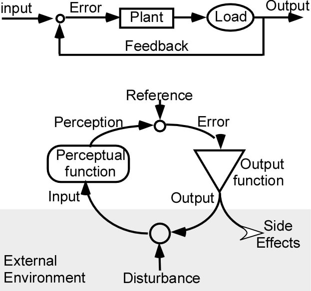
EJ: As was noted by others, PCT primarily uses a form of PI (Proportional,
Integral) function as its output, rather than a PID function (which adds the
derivative component.) This means most of the gain in a typical PCT control
loop is incorporated into the output term, although there are placeholders for
environmental feedback function gain and perceptual input function gain. The
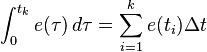
output term is also typically made discrete, and thus uses an integrating
rather than an integral function. We call it a “leaky integrator.” One of
the side effects of the leaky portion, I believe, is to leave a small residual
error – what the Wikipedia article calls “droop” – because proportional
controllers require non-zero error to stay operative…
RM: This is a excellent post, Erling. Clear, concise and accurate! You seemed to me channeling Bill Powers when you wrote it. Thank you.
RM: I will just add that it is very difficult to say what PCT can contribute to robotics since PCT is the application of control theory to the reverse engineering of control systems that have already been “built”: mainly living control systems. But all the things you mention are useful ideas for the builder of control systems, particularly the idea of basing construction of the robot on an architecture that is a hierarchy of control systems. I think that’s what Rupert has been doing with his little demo robots. His robots may not control the lower level perceptions as well as other robots but his robot controls a higher level perception – a sequence, I believe – and the sequence is indeed a controlled perceptual input, not just a pre-programmed sequence of outputs. If the sequence is disturbed the robot goes back to the point where it left off to complete the sequence. Rupert’s robot is a pretty impressive demonstration of PCT, I think!
Thanks again, Erling, for this wonderful post. Definitely a keeper. Like Kent, I am \also glad to know that you are contributing a chapter to LCS IV.
PS. OK, I will just say that your only mistake – a trivial and irrelevant one – was to say that force is integrated acceleration. Force is proportional actually proportional to acceleration – F = ma – the constant of proportionality being the mass of the object being accelerated.
Again, super post Erling.
EJ: The chief advantage of the PCT approach, to my mind, is to provide what
the article calls “cascaded PID control.” This is a way to get better dynamic
performance from linear PID controllers. The key idea is that the output of
one PI(D) controller provides the set point reference for another PI(D)
controller. This is a prime feature of Hierarchical PCT. There seem to be
several distinct benefits from this approach.
EJ: 1) Additional degrees of freedom. Parameters are not collapsed into a
single equation, driving control of a single process variable. Rather, there
is finer-grained control of more than one perception.
EJ: 2) Differential time constants. The article clearly describes how the
outer loop has a long time constant, while the inner loop can respond much
more quickly. HPCT expands on that concept even more, by providing multiple
inter-nested loops, with progressively shorter time constants when descending
the hierarchy. This partitions the overall control task, and improves overall
dynamic performance.
EJ: 3) Reducing or eliminating recourse to feed-forward (open-loop) control.
When some of the time constants in item (2) above are extremely fast, there
may be less need for internal models to predict the effects of system
characteristics or of future disturbances. Such variables can be handled
directly, in real time, by closed-loop feedback control. Essentially the
environment is allowed to model itself.
EJ: 4) Differential tuning to the physics at different points in the process.
Having different PI controllers tuned to different perceptions (what the
article calls “process variables”) allows a better approximation of the
physics applicable to each one.
EJ: 5) Partitioning the perceptions themselves. When PCT uses cascaded
control, it does not simply measure the same variable at two different spots,
(which is the example offered in the Wikipedia article.) PCT attempts to have
a lower loop control a constituent perception of a higher loop, as a means of
its own implementation. The result is that the control task for the higher
loop is simplified. Fast-changing dynamics from disturbances are handled at a
lower level, while the higher level monitors a different and slower overall
measure of the results of control.
EJ: An example of (5) would be Powers’ PCT simulation of control of an
inverted pendulum. If I am remembering the details correctly, Position
control of the bob supplies the reference for Velocity control of the cart,
since position is integrated velocity. Velocity control supplies Acceleration
control of the cart, since velocity is integrated acceleration. Acceleration
control supplies the reference for Force control against the cart, since
acceleration is integrated force.
EJ: 6) Graded changes of reference. Cascaded PI control seems to get away
from step changes in the set points, which do not seem very plausible
biologically anyway. This is akin to what the article calls "set point
ramping."
EJ: An interesting case can be made with regard to derivative control, by
incorporating the rate of change of the error over time. This is meant as a
predictive approximation of future error, to refine overall stability of the
system. Standard PCT control loop equations do not seem to include this form
of control, although in HPCT the rate of change of any variable in itself can
become an object of perception, which we call Transition control.
EJ: However, I would make the case that in human control systems at least,
the Emotional system of the body is connected to the rate of error change over
time. I am not sure over how broad a scale the error would be measured. But
different emotions may well correlate with the slope of error change, and
whether it is rising or falling. The output of such a system seems to make
broad systemic changes in the body, albeit reversible and subject to decay
over time.
EJ: These changes seem to affect performance characteristics of the body. As
such, this is more like altering parameters of control, or the gain parameter
itself. This may be a form of Derivative control, operating on a systemic
basis, rather than for individual control loops. Alternatively, it may be a
form of what the Wikipedia article calls “PID gain scheduling,” where
parameters are adjusted to different operating conditions.
EJ: The above list of advantages seems to be a decided plus when it comes to
the form of negative feedback control incorporated into Perceptual Control
Theory. Yes, it is based on PID control, or at least PI control. But it is
primarily a form of cascaded PI control, which confers a host of benefits.
EJ: Hope this is helpful. BTW, I expect to utilize some of the above wording
and formulations in the article I am writing for the Living Control Systems VI
edited book.
All the best,
Erling