I did it long ago and don’t have the simulation. So I cobbled together a new spreadsheet that shows that this is true. The spreadsheet is here. The spreadsheet shows that your predicton holds for the two coefficients you mention (.9 and1.1) and, more generally, for all possible coefficients of x and y for person B in the conflict. That is, the spreadsheet shows that the the virtual variable that is always controlled when A controls the variable x + y and B controls the variable k1x+k2y is ((1+k1)/2)*x + ((1+k2)/2)*y. It also shows that this is true regardless of the reference values for x and y.
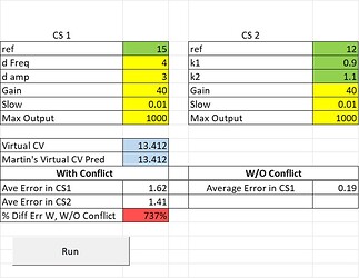
Here is a display of the results that you will see when you open the spreadsheet:
There are two control systems: CS1, which is controlling x+y, and CS2, which is controlling k1x + k2y. The values for k1 and k2 can be set by entering values into the green cells to the right of k1 and k2. They are currently set to the values you suggested, .9 and 1.1. But any two values will work.
The value in the cells colored yellow are parameters of the control systems. They can be varied but I would leave them alone for now until you get used to using the spreadsheet. The current parameters define two control systems of equal ability (gain and slowing) with the same limit on the amount of output that they can generate.
The values in blue are the actual (computer) value of the virtual controlled variable (labeled “Virtual CV”) that emerges from the conflict and your predicted value of that variable (labeled “Martin’s Virtual CV Pred”) per the equation above: ((1+k1)/2)*x + ((1+k2)/2)*y. The values are always identical,confirming Martin’s predition. This shows that when two control systems control two differnet functions of the same environmental variables (x and y) the result is a virtual controlled variable whose value is midway between the values desired by each control system.
Although this spreadsheet shows that it is possible to make a very accurate prediction of the value of a virtual controlled variable that emerges from the interation between two control systems controlling different perceptions of the same environmental variables, can’t think of a real world example of phenomenon that corresponds to what the moel is doing. Well, maybe arm wrestling and tug of war.
Neverltheless, I think the spreadsheet was worth developing because it nicely demonstrates my point about the existence of significant error in the individuals that make up a collective (in this case, a collective of two indivisuals) keeping a virtual controlled variable in a reference state that differs from the reference states of the indiividuals in the collective. This can be seen by pressing the “Run” button, which automatically runs a conflict between CS1 and CS2 with those two control systems controlling x+y and k1*x+k2y, respectively, relative to different references, and then does a run with CS1 controlling x+y on its own.
The results are shown oin the table just above the “Run” button. The table shows the size of the error signal (in units of neural current) in CS1 (and CS2) when they are in conflict and when CS1 is controlling on its own. The percentage increase in the size of the error experienced by CS1 when in conflict versus when controlling alone is shown in the cell colored red. The table above shows that when the two conrol systems are in conflict , controlling relative to fairly different references (15 and 12) CS1 is experiencing over 700% greater error while maintaining the virtual controlled variable in its reference compared to when CS1 is controlling without the conflict.
In real life, error corresponds to pain in the form of stress and anxiety. The spreadsheet shows that the pain experienced when in a conflict can be a very high price to pay for keeping some variable in a stable virtual reference state.
Best, Rick
