Statistics: what is it about? Bayes Episode 2

[Martin Taylor 2009.01.04.15.32]

Following on from …

Martin
Taylor 2009.01.03.22.54]

Which should be understood before reading the new material. I repeat
some of it…

  1. All probabilities are subjective in the sense that they depend on
    the background knowledge of the observer. The background knowledge may
    include models, records of previous occurrences of the “probabilistic”
    matter, pure intuition, faith, and anything else you can think of.
    “Frequentist” probability, on which significance statistics are based,
    takes into account only records of previous occurrences (but see below
    for a problem with even this).

  2. All probabilities are conditional. That’s part of the background
    knowledge that you bring to bear. In the “frequentist” view of
    probability, you look at N situations, and say that on M of them the
    event E happened, so the probability of event E happening the next time
    is M/N. But that’s not legitimate, You should at the very least say
    “conditional on the N situations all having the same characteristics
    insofar as event E is concerned, and on the next occurrence of the
    situation it will also have those characteristics.” In physical fact,
    no two of the N situations had all the same characteristics. At the
    very least, the universe had a different age when each occurred.


What
you can say about the “White Swan” problem is that if the conditions
remain the same, the likelihood that the next swan you see will be
white increases the more swans you have seen without seeing a non-white
one. Let’s consider some hypotheses about that. Say we have been
observing swans and they have all been white. We know little enough
about the background of these swans that we are prepared to say the
conditions will be considered to be “the same” the next time we see a
swan, any swan. The hypotheses we will consider are

H1: No swans are white.

H2: Half of all swans are white

H3: 75% of all swans are white

H4: All swans are white.

That’s what we did in Episode 1. We found that if we had no initial
preconceptions about the proportion of swans that are white, we could
find posterior probabilities for the four hypotheses given that we had
seen 10 swans and all of them were white. These four hypotheses were
samples from an infinite set of hypotheses of the same type, the
hypotheses differing only in the value of a single parameter:

Hx: The proportion of swans that are white is x (0 <= x <= 1.0).

In other words, given that we have seen a bunch of swans (we will keep
10 as the example), what is the (subjective) likelihood of the
hypothesis? We will see that in this case we can’t specify a subjective
probability for any single hypothesis (all of them must be
infinitesimal), but we can find a total probability for hypotheses
within a range of values of x.

from Episode 1, we had:

After
seeing 10 swans which were all white, we can compute the likelihoods
from the initial formula rather than recomputing new prior
probabilities, but we can simplify by ignoring p(D) because it always
falls out from the comparisons. D in this case is the observation of 10
swans, not just of the tenth swan.

L(H1|D) = 0.25 * 0 = 0

L(H2|D) = 0.25 * (0.5)^10 = .0002

L(H3|D) = 0.25 * (0.75)^10 = .014

L(H4|D) = 0.25 * 1 = 0.25

Normalizing so that the probabilities sum to 1.0, the posterior
probabilities are

p(H1|D) = 0

p(H2|D) = 0.0009

p(H3|D) = 0.053

p(H4|D) = 0.947

By this point, the initial prior distribution has become almost
irrelevant.

This is an important point, because most critiques of Bayesian analysis
centre on the difficulty of setting up “correct” prior probabilities.
It is, in principle, impossible to set up “correct” prior
probabilities, because they depend on what each person believes or
assumes before making the observations.

I am not sure, but I think I first appreciated the way data overwhelm
the “prior problem” when I read Satosi Watanabe’s magnificent “Knowing
and Guessing: A formal and quantitative study” (Wiley, 1969). If you
haven’t read that book, I highly recommend it. For me it was one of
very few books that have seriously changed my way of thinking (others?
B:CP, of course, W.R.Garner “Uncertainty and Structure as Psychological
Constructs”, Wiley 1962, which I read in manuscript while I was
Garner’s student, Norbert Wiener’s “Cybernetics” – not “The Human Use
of human Beings”, and Von Neumann and Morgenstern’s “Theory of Games”
which I read when on a transcontinental train trip as a member of a
cricket team going to an Inteprovincial tournament in Vancouver. There
were probably others, but those are the ones I remember best).

Back to the chase. Now, for any value of x, the hypothesized likelihood
that a random swan (or equivalently in this case, the very next swan)
will be white, we can say that L(Hx|D) = x^10. Here is a graph of x^10
for x between 0 and 1.0. The curve shows the relative likelihood of the
hypotheses shown on the x-axis. To get the posterior probability
distribution, one must multiply one’s prior probability distribution
point by point with the values on this curve.

x_10.jpg

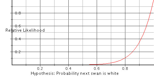
This is a graph of the relative likelihoods of all the infinite number
of possible hypotheses, scaled so that the maximum value is unity. Any
other scaling would be permissible, since all that matters is the
amount by which one hypothesis is more credible than another. For
example, after seeing these 10 white swans, the hypothesis that 95% of
all swans are white is 1.71 times as likely as that 90% are white, and
0.6 times as likely as that all swans are white.

After getting the data that these first 10 swans were white, you can
adjust your subjective probability that the next swan will be white by
multiplying your prior probability for any given hypothesis by the
value on this curve. As we did in part 1, you then must scale so that
the integral of the resulting curve is 1.0 (or the sum, if you had a
finite prior probability for only a finite set of initial hypotheses,
rather than the continuum implied by the likelihood curve).

Remember that these likelihoods are all subjective, and are all
conditioned on certain presumptions, notably that the swans we have
seen are representative of all swans, and that we are as likely to have
seen any one individual swan as any other. If you have other
conditionals, your likelihoods might change. For example, you might
have an initial assumption that all swans in a flock are the same
colour, but the colour changes from flock to flock, and you might have
come to believe that all the swans you have seen so far belong to the
same flock. Then observing 10 swans would give no more information than
observing one.

The conditionals are where all the problems arise with data sampling.

Now let’s consider what happens to our hypotheses if the eleventh swan
we see happens to be a black one. Continuing the analysis as before, we
would have:

L(Hx|D) = x^10 * (1-x)

We have ten white swans, and one black one. What conditionals are we
considering? That the black and the whites are all just swans, one as
likely as the other to come into view? That the black swan is the
forerunner of a new flock of black swans? And what hypotheses are we
asking about? “What is the probability that the next swan we see will
be white”? Or “What is the proportion of white swans among all swans?”
These considerations did not appear when all the swans we had seen were
white, but now we have a distinct difference among possible
probabilities:

  1. p(next swan is white | all swans are equally likely to be seen)

  2. p(next swan is white | swans fly in flocks all of the same colour)

  3. p(a randomly chosen swan is white | all swans are equally likely to
    be seen)

  4. p(a randomly chosen swan is white | swans fly in flocks all of the
    same colour)

We now have the data sampling question laid out baldly. Is one swan as
good as another, or are there subpopulations distinguished by flocking
together? We have as yet no evidence one way or the other, but we can
compute the subjective probabilities of the two distinct events “the
next swan will be white” and “a randomly selected swan will be white”,
where “random” means that we have no evidence that the manner of
selecting the swan affects the result of the choice.

On the evidence at hand (ten white swans and one black one) we also
have an important question: “Does the order in which we saw the swans
matter?” Here’s why.

If we just know the numbers and not the order, there are eleven
different sequences of swan colour we might have observed, whereas if
we do know the order, there is only one. For the conditional “all swans
are equally likely to be seen”, the probabilities are similarly
affected for all the hypotheses, so the order doesn’t matter. The
probabilities for questions 1 and 3 are the same.

But if you assume (i.e. use the conditional) “swans fly in flocks all
of the same colour” the order of their arrival does matter. If the
black swan was the first you saw after you started counting, under your
assumption it must have been the last member of a black flock; if it
was the last one you counted, then under your assumption it is the
first of a black flock (meaning that you may have a rather high prior
probability that the next swan will be black, even though a flock might
have only one member, and despite the fact you have just seen 10 white
swans in a row before the black one); and if it is in the middle
somewhere, you have seen three flocks, two of them white, one black,
and the black flock has only one member. So, the likelihoods change. In
the first two cases, the likelihoods are the same as they would be if
you had seen one white and one black swan, whereas if the black swan
was in the middle of the order, the likelihoods would be as though you
had seen two white swans and one black. In all these cases, the
probabilities for questions 2 and 4 are different, and both are
different from those applicable to questions 1 and 3.

Furthermore, if you happen to want also to test hypotheses about the
distribution of flock sizes, and the black one was in the middle, then
with the conditional that swans always fly in flocks of a common
colour, you have evidence: flocks can be as small as one, and as large
as the longest sequence of whites that you have observed. The point is
that the same data can be used to adjust likelihoods on quite different
kinds of hypotheses, depending on the conditionals that you use (the
beliefs that you are willing to take as assumptions when making your
judgments).

However, let’s get back to the four different questions above, using
the conditional “all swans are equally likely to be seen”. If the
probability of seeing a white swan is hypothesized to be x, then for
consistency you must also take the probability of a non-white swan to
be 1-x. (If you don’t, then your belief level must be remapped onto the
number scale for it to be treated as “probability”). So, setting aside
the fact that there are eleven different possible orderings of where in
the sequence the black swan came, we have, as mentioned above:

L(Hx|D) = x^10 * (1-x),

and to save time later, I note that if we had 20 white swans and 2
black ones,

L(Hx|D) = x^20 * (1-x)^2

Here are the relative likelihood curves for the initial 11 observations
and for all 22, scaled so that the peak is set to 1.0.

x_10-1_20-2.jpg

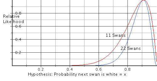
More data simply concentrates the likelihoods of the different
hypotheses. For example, if you would have bet 5 to 3 on the
probability that the next swan would be white being 0.91 rather than
0.8 after 11 swans, you would bet at a bit more than 5 to 2 after
seeing 22 swans. However, if your bet had been between hypotheses that
the probability was either 0.8 or 0.7, your appropriate odds would have
been about 12 to 5 after 11 swans and about 6 to 1 after 22 swans.

In other words, what you can do with these likelihood curves is
estimate how much the credibility of any hypothesis has changed when
compared to the credibility of any other hypothesis. They don’t tell
you what you should have as a subjective probability of any specific
hypothesis, because that depends on what other evidence you might have
from models, faith, intuition or anything else – the evidence that
gave you your prior probabilities.

But as we saw in episode 1, after you get a reasonable amount of data,
your priors don’t matter very much unless they were very strong. Given
these data on swans, you would have had to have a very compelling prior
probability that black and white swans were equally likely, in order
rationally to hold onto that view in the face of these data. People
can, of course, be irrational, and often are. These curves, however,
represent the most that anyone could get out of the data given the
conditionals on which the analysis was based. They represent the ideal
performance for these data with those conditionals.

In the handwritten seminar notes on “Bayesian Analysis, Information,
and Signal Detection”
and
, the
likelihood curves above are called the “Likelihood Gain Function”, and
the related curves of posterior probability are called the “Assessment
Function”.
Enough for this episode. I think episode 3 may deal with the sampling
problem and/or distinguishing among populations, but we shall see. I
may have a different idea by the time I get to it. For now, I’m tired
and I’m going to bed :slight_smile:
I hope these notes are being more helpful than confusing.
Martin

···

http://www.mmtaylor.net/Academic/Bayesian_Seminar_1.PDFhttp://www.mmtaylor.net/Academic/Bayesian_Seminar_2.PDF

[From Rick Marken (2009.01.04.1110)]

Martin Taylor (2009.01.04.15.32) --

Following on from ...

Martin Taylor (2009.01.03.22.54)--

This is all very exciting. But what in the world does it have to do
with understanding purposeful behavior (control)?

Best

Rick

···

--
Richard S. Marken PhD
rsmarken@gmail.com

[From Bill Powers (2009.01.06.1222 MST)]

Rick Marken (2009.01.04.1110) –

Martin Taylor
(2009.01.04.15.32) –

Following on from …

Martin Taylor (2009.01.03.22.54)–

This is all very exciting. But what in the world does it have to do

with understanding purposeful behavior (control)?

I don’t think we can just “do PCT” and ignore everything that
everyone else believes and is interested in. That’s the monastic
approach: shut the doors and keep the world out. Unfortunately, the doors
not only shut the world out, they shut you in, and you will pass from the
scene unnoticed, having wasted all your life impressing a few brethren in
the faith who will also disappear without a trace.
I think life is applied PCT. If we don’t understand what others are doing
and are trying to achieve, we’re only showing that the theory needs more
work. You don’t get people to change their behavior by saying “Stop
doing that.” Nor can we simply assume naively that it’s their
behavior that needs changing.

Best,

Bill P.

[Martin Taylor 2009.01.06.14.30]

[From Rick Marken (2009.01.04.1110)]

Martin Taylor (2009.01.04.15.32) --
Following on from ...
Martin Taylor (2009.01.03.22.54)--
This is all very exciting. But what in the world does it have to do
with understanding purposeful behavior (control)?

If you understand Bayesian logic and see a use for it, use it. If you
either don’t understand it, or do understand it and don’t see a use for
it, then ignore it.

whether someone was controlling perimeter or area, for example, or in
the computer-based discovery of what someone was controlling for. The
results might have been no better than the results you achieved, but if
that was the case, it would show that your methods were optimal.

I’m trying to achieve two things with this series of notes: (1) to get
people to understand that there is a limit to what can be gained from
given data, and that this limit is independent of mechanism, whether it
is in a computer or in a neuron or in a brain; and (2) that there are
other ways of getting at the mechanisms of control than brute force
comparisons.

To find out what people are controlling for in a particular situation
is what you most want to do. That involves making hypotheses about what
they might be controlling for, and gathering data that seem relevant to
the question. The situation is appropriate for assessing the relative
probabilities that one or another hypothesis might actually represent
what is happening inside the person. To do that in a Bayesian manner is
appropriate if you can define your hypotheses and the appropriate
conditionals well enough to suit yourself. But you can use other
techniques to your heart’s content. Often another method is easier to
do, and ease of use often offsets any potential gain in efficiency.

So, if you want to use Bayesian methods, be my guest. If you don’t,
then don’t.

Martin

···

from my side, I would have seen a use for it in your experiment on

[From Rick Marken (2008.01.06.1145)]

Bill Powers (2009.01.06.1222 MST)

Rick Marken (2009.01.04.1110) --

This is all very exciting. But what in the world does it have to do
with understanding purposeful behavior (control)?

I don't think we can just "do PCT" and ignore everything that everyone else
believes and is interested in.

I was asking how this was related to control, not saying that it
shouldn't be discussed. I see that Martin understood my question so
I'll reply to him in a second.

Best

Rick

···

--
Richard S. Marken PhD
rsmarken@gmail.com

[From Rick Marken (2009.01.06.1200)]

Martin Taylor (2009.01.06.14.30) --

From my side, I would have seen a use for it in your experiment on whether
someone was controlling perimeter or area, for example, or in the
computer-based discovery of what someone was controlling for. The results
might have been no better than the results you achieved, but if that was the
case, it would show that your methods were optimal.

That sounds great. Could you explain how the Baysean version of my
"computer-based discovery of what someone was controlling for" (which
is just an application of "the test for the controlled variable")
works. I'd love to be able to improve the algorithm!

Best

Rick

···

--
Richard S. Marken PhD
rsmarken@gmail.com

[Martin Taylor 2009.01.06.15.37]

[From Rick Marken (2009.01.06.1200)]
Martin Taylor (2009.01.06.14.30) --

From my side, I would have seen a use for it in your experiment on whether
someone was controlling perimeter or area, for example, or in the
computer-based discovery of what someone was controlling for. The results
might have been no better than the results you achieved, but if that was the
case, it would show that your methods were optimal.
That sounds great. Could you explain how the Baysean version of my
"computer-based discovery of what someone was controlling for" (which
is just an application of "the test for the controlled variable")
works. I'd love to be able to improve the algorithm!

If you specify your background assumptions (the conditionals) and the
kind of data you would expect from each of your competing possibilities
(hypotheses), then it can be done. There’s no guarantee it would
improve the algorithm, though, since the existing algorithm might
already be optimal.

Perhaps it would be better to wait an episode or two, until I get into
discriminating among hypotheses. Perhaps you can extrapolate that for
yourself from episode 2, but I hope it will become clearer shortly.

Martin

[From Rick Marken (2008.01.06.1415)]

Martin Taylor (2009.01.06.15.37) --

If you specify your background assumptions (the conditionals) and the kind
of data you would expect from each of your competing possibilities
(hypotheses), then it can be done.

OK, let's do it for the "mind reading" demo at

Mindreading.

The background assumption is that the 2 dimensional screen position of
one or none of the three characters is under control at any particular
time. There are, thus, 4 competing possibilities:

Hypothesis 1. Homer's position is under control
Hypothesis 2. Bart's position is under control
Hypothesis 3. Lisa's position is under control
Hypothesis 4. No one's position is under control

The data I use to decide which hypothesis to accept as true is the
correlation between the disturbance to a character's 2 D position and
the character's actual 2 D position. I will refer to this correlation
as r.dp(c), where c is the index for the character (c=h for "Homer",
c=b for "Bart", etc). So the data I expect for each of the 4
hypotheses is as follows:

Hypothesis 1. r.dp(h)<<r.dp(b) and r.dp(h)<<r.dp(l)
Hypothesis 2. r.dp(b)<<r.dp(h) and r.dp(b)<<r.dp(l)
Hypothesis 3. r.dp(l)<<r.dp(h) and dp(l)<< r.dp(b)
Hypothesis 4. r.dp(h) = r.dp(b) = r.dp(l)

I am guessing that Baysean statistics might be able to help me out if
I have some reason to believe that the a priori probability of
controlling the position of one character is greater than that for
another character. But I don't have any reason to believe this.

So tell me how Baysean statistics might be able to help me out here.

Best

Rick

···

--
Richard S. Marken PhD
rsmarken@gmail.com

[Martin Taylor 2009.01.06.1745]

Responding to a message Rick posted last year, that just arrived

[From Rick Marken (2008.01.06.1415)]
Martin Taylor (2009.01.06.15.37) --
If you specify your background assumptions (the conditionals) and the kind
of data you would expect from each of your competing possibilities
(hypotheses), then it can be done.

OK, let's do it for the "mind reading" demo at
.

I tried to run your demo to get some data to make it real, but I found
I was unable to influence the movements of any of the characters. They
all started off moving reasonably rapidly from the bottom of the
display, and “random walked” around the window getting slower and
slower until they all converged in the middle. Does it work on-line for
you, and if so, what browser and operating system? I tried with Firefox
3 under Mac OS X 10.5.6.

I started to do a Bayesian analysis on your problem with explanations
as to how it all worked, but it seemed to be becoming one of my
tutorial sessions. So I will answer as part of episode 4 or 5, probably
4. That might make it more generally relevant.

Martin

···

http://www.mindreadings.com/ControlDemo/Mindread.html

[From Rick Marken (2009.01.07.2210)]

Martin Taylor (2009.01.06.1745]

I tried to run your demo to get some data to make it real, but I found I was
unable to influence the movements of any of the characters. They all started
off moving reasonably rapidly from the bottom of the display, and "random
walked" around the window getting slower and slower until they all converged
in the middle. Does it work on-line for you, and if so, what browser and
operating system? I tried with Firefox 3 under Mac OS X 10.5.6.

It works well on every browser I've tried on PCs (Windows or Vista).
It does work lousily with Firefox on the Mac (it's very jerky for me).
It works much better in Safari for some reason, but you have to push
the mouse button to get the applet to "hear" the mouse movements. When
you press the mouse button you will also see the correlations; you can
make them disappear (or reappear) at will by toggling the mouse
button. But you probably want to leave the correlations on since
that's the data you need.

I started to do a Bayesian analysis on your problem with explanations as to
how it all worked, but it seemed to be becoming one of my tutorial sessions.
So I will answer as part of episode 4 or 5, probably 4. That might make it
more generally relevant.

Goody. I can hardly wait.

Best

Rick

···

--
Richard S. Marken PhD
rsmarken@gmail.com

[Martin Taylor 2009.01.08.10.46]

[From Rick Marken (2009.01.07.2210)]

Martin Taylor (2009.01.06.1745]
I tried to run your demo to get some data to make it real, but I found I was
unable to influence the movements of any of the characters. They all started
off moving reasonably rapidly from the bottom of the display, and "random
walked" around the window getting slower and slower until they all converged
in the middle. Does it work on-line for you, and if so, what browser and
operating system? I tried with Firefox 3 under Mac OS X 10.5.6.
It works well on every browser I've tried on PCs (Windows or Vista).
It does work lousily with Firefox on the Mac (it's very jerky for me).
It works much better in Safari for some reason, but you have to push
the mouse button to get the applet to "hear" the mouse movements.

Thanks. I run Windows XP Pro on my Mac under Parallels 4, so maybe I’ll
try it with Firefox there (and if not there, I’ve just last night
installed Ubuntu Linux, and that might work). Actually, my problem
wasn’t that anything was jerky. Everything moved smoothly, but was
totally unresponsive to the mouse. Also, is it to be expected that the
characters move slower and slower during the course of the run,
restricting their movements to an area that converges toward the
centre, where they all settle at the end of the run, before restarting
at the bottom of the window?

When
you press the mouse button you will also see the correlations; you can
make them disappear (or reappear) at will by toggling the mouse
button. But you probably want to leave the correlations on since
that's the data you need.

Actually, as soon as you say that, you put a conditional on the Bayes
analysis “Given that the data consist of the correlations”. I’ll work
with that, but I kind of hoped there might be some access to the four
tracks, since that would give much more scope for the analysis. You
could test hypotheses about the parameters of the person’s control
system, for example, or look to see whether you could detect changes
during the run as to whether they were controlling and/or whether they
switched which character they were controlling.


I started to do a Bayesian analysis on your problem with explanations as to
how it all worked, but it seemed to be becoming one of my tutorial sessions.
So I will answer as part of episode 4 or 5, probably 4. That might make it
more generally relevant.
Goody. I can hardly wait.

I hope it meets your expectations. As I said before, it’s not
guaranteed to come up with anythng better than what you do. It might
just say you are already doing the best you can with the data, but I
suppose that in itself would be worthwhile. We shall just have to see.

Martin

[From Rick Marken (2009.01.08.1950)]

Martin Taylor (2009.01.08.10.46)--

. Also, is it to be expected that the characters move slower and
slower during the course of the run, restricting their movements to an area
that converges toward the centre, where they all settle at the end of the
run, before restarting at the bottom of the window?

Yes. That happens when the mouse has no effect on the position of the
characters, as was the case with you. It happens because the screen
position (x) of each character is determined by the formula x = d - km
(where d is the disturbance, m is the mouse position) rather than just
x = d - m. The value of k is inversely proportion to the absolute size
of the correlation between x and d. This correlation will tend to be
low when a character is controlled. So when a charter is not under
control (as is true for all characters when the mouse has no effect)
the effect of the mouse of the position of the character is
exaggerated. I do this to make it harder for an observed to tell which
character is under control. If I did not do this the controlled
character, if it is being moved in an arbitrary pattern on the screen,
would stand out as the character that is moving around the the least.
With this little trick the screen movements of the controlled
character resemble those of the uncontrolled ones.

Actually, as soon as you say that, you put a conditional on the Bayes
analysis "Given that the data consist of the correlations". I'll work with
that, but I kind of hoped there might be some access to the four tracks,

There are only three tracks and they are certainly available if you need them.

Best

Rick

···

--
Richard S. Marken PhD
rsmarken@gmail.com