[From Richard Kennaway (2017.10.13 1448 GMT)]
Thanks, Warren, for prodding me to take a look at this.
I've read Rick's paper, and some of the background papers, but not yet Zago et al's response or most of the rather vituperous discussion on CSGNET. These are just a few preliminary notes, but if I wait until I know everything I want to say on the subject I'll never post anything.
1. Several people in the discussion are in error about the meaning of a mathematical equality, or a law of physics expressed as one. No such equation expresses any sort of causal relationship.
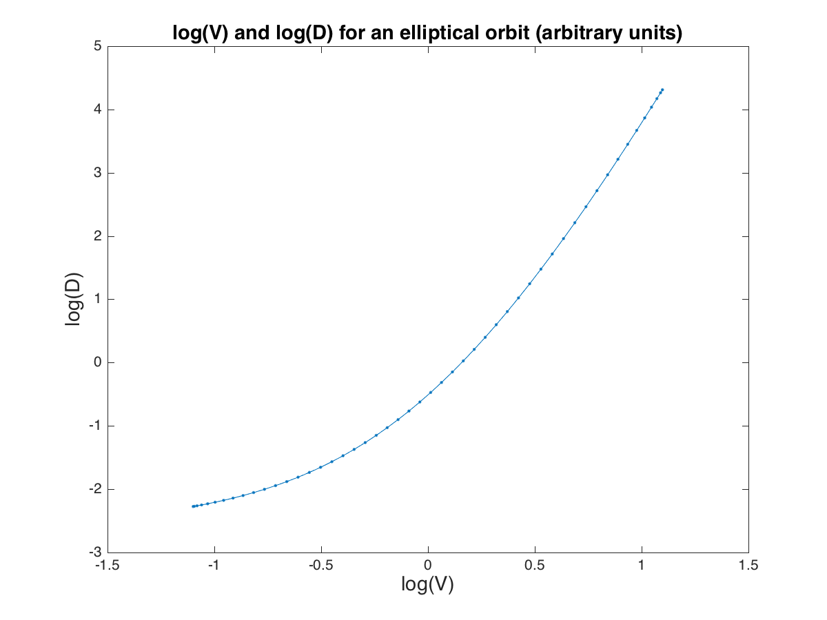
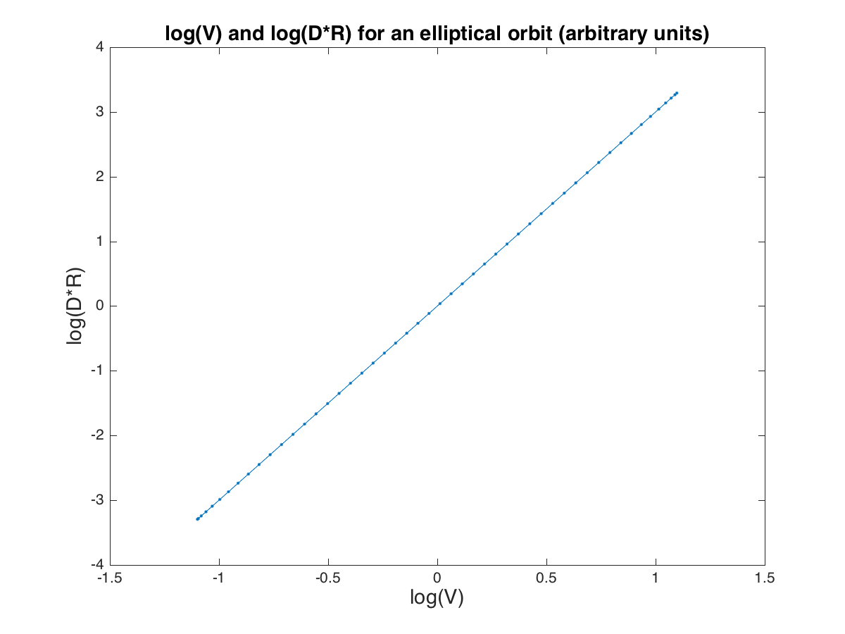
For any smoothly traversed curve in a plane, we have V = D^(1/3) R^(1/3), where V is the speed, R the radius of curvature, and D the magnitude of the cross product of acceleration and velocity. This is simply a mathematical fact. We can equally well arrange the equation as D R = V^3, R = V^3/D, etc. All of these forms mean the same thing. None of them imply any causal relationship among the variables, any more than the expression 2+2 causes 4 or 4 causes 2+2.
One of Newton's laws is F = M A, force equals mass times acceleration. This can with exactly the same meaning be written in any mathematically equivalent way, such as M A = F, M = F/A or A = F/M, or F - M A = 0. This is not, contra [Dag Forssell 2017.11.12 19:45 PST], something that engineers do but really shouldn't. All of these equations mean the same thing. If one is true, all are true. Certainly you can apply a force to a mass to cause an acceleration, and cannot apply a force to an acceleration to produce a mass, but those causal facts have nothing to do with any way of writing F = M A. Consider also the more drastic rearrangements of Newton's laws that are the Lagrangian and Hamiltonian formulations. All of these describe the same physical reality.
In physics, none of the equations mean that the left hand side is caused by the right hand side. If you seek causality in physics, look for it in the properties of its differential equations, that allow the future to be calculated from the present. These properties have nothing to do with which terms happen to be on the left hand side of an equals sign.
[Digression: in econometrics there is something called an SEM (Structural Equational Model). This is a set of equations whose left hand sides are single variables, and which are intended to be read with causal meaning: the things represented by variables appearing on the right hand side are asserted to cause the thing represented by the left hand side. However, some SEM modellers are confused about this and do not clearly distinguish between the causal and non-causal reading of an equation. They might be helped by using different symbols for the different concepts, instead of the equals sign for both. I mention this just in case anyone in this discussion is familiar with SEMs. In the present discussion, none of the equations should be read causally.]
2. As mentioned above, V = D^(1/3) R^(1/3). This mathematically implies that if any two of these variables have a power-law relationship with each other, they each have power-law relationships with the third. However, no power-law relationships need be present at all.
3. If D is constant, V is proportional to R^(1/3). This is the classic power law. Conversely, the classic power law implies that D is constant. However, actual power laws in the literature have widely varying exponents. The 1/3 power, despite frequent citation, does not seem to play any special role.
4. Physically, a particle can be made to move along any path with any course of velocity over time, independently of the curvature of the path. For such an arbitrary course of velocity, the power law in general does not hold. When the power law does hold, this is a non-trivial fact about the motion. It is not guaranteed mathematically. When it does hold, the exponent can take any value. If in some class of situations the exponent is always found to be close to 1/3 (equivalently, that D is approximately constant), this is a further non-trivial fact.
5. If experimental data are obtained for V and R (from which D can be calculated), then any subset of those data selected for having a single value of D must mathematically obey the power law. This is true regardless of the source of the data and the mechanism that produces the data. The power law is only non-trivial if no selection on D is made. If the power law is then observed, this is a nontrivial fact. So I disagree with Rick's characterisation of the power law as omitted variable bias.
6. An empirical regularity can rule out models that do not exhibit the same regularity, but cannot distinguish models that do. Many completely different models might give rise to the same observations.
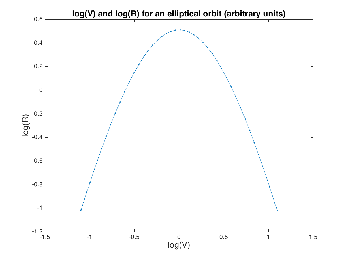
7. Consider simple harmonic motion in two dimensions. The general path is an ellipse. Let its semi-axes be P and Q. Taking these to be the coordinate axes, the path is x = P cos(wt), y = Q sin(wt) where w is the (abstract) angular velocity (not to be confused with the angular velocity of an object moving like this) and t is the time.
I calculated that for this example, the value of D is constant, in fact equal to A B w^3. Constant D implies the power law. Thus two-dimensional harmonic motion always satisfies the power law, regardless of the mechanism.
Suppose you swing your arm, using only the shoulder joint, so that the hand describes a small ellipse at a moderate velocity, with none of the muscles working very hard, relative to their tension when the arm is held still. With all the relevant variables being small, we may expect a linear analysis of the mechanism of this system to be reasonably accurate. This linearity implies that the hand must be performing simple harmonic motion in two dimensions. But as just seen, two-dimensional SHM necessarily obeys the power law, regardless of mechanism. Therefore an experiment studying this type of movement would offer no insight into the mechanism.
8. A particle moving with constant linear velocity along a path of varying curvature satisfies a power law, although of a degenerate sort: both exponents are zero. V = K D^0 R^0 where K is constant. This is not the sort of power law generally found in these experiments.
9. A pendulum swinging in a single plane (an example used by one of Rick Marken's interlocutors), or a weight bobbing up and down on a spring, do not satisfy the power law. R is constant in both situations, while V varies. No tuning of the alpha parameter can produce plausibly straightish lines on a log-log plot.
10. Something immediately struck me as fishy about the power law, because it predicts that a straight line is traversed at infinite velocity. So I looked up Gribble and Ostry and found that the measure of radius that they use is not the actual radius R, but R* = R/(1 + alpha R), where alpha is a constant parameter. This is close to R when R is much smaller than alpha, and approaches 1/alpha as R tends to infinity.
This strikes me as something of a fudge. There are many ways in which we can impose a ceiling on R*; why this one? One might equally well choose, for example
R* = (2/(pi*alpha))*atan(pi*alpha*R/2)
or
R* = (1/alpha)*tanh(alpha*R)
Both of these have the property of tending to R for small R and to 1/alpha for large R.
I could suppose that the experiments are all in the range of small R, but then there would be no need to introduce alpha, and G&O mention the power-law being observed for lemniscates (figure 8s). In these, if the curvature varies smoothly along the path, it must go to zero at least twice. So in some experiments, at least, alpha must play an essential role in bounding the predicted velocity. I would like to see how closely the power law fits the data when R is comparable to 1/alpha or greater, for each of these three definitions of R*.
It has been quipped that any data looks like a straight line when plotted on log-log paper. This is an exaggeration, but with this extra parameter alpha to fit, I wonder. On the other hand, G&O do find remarkably high correlation coefficients, on a par with those found in PCT experiments. So it does look, prima facie, as if their data non-trivially fit the power law.
G&O do not fit alpha, but use values from Viviani & Stucchi 1992, who do fit alpha to their data. I don't know why G&O didn't fit alpha to their own data -- it is not a global fundamental constant, since they use different values in different experiments.
G&O allow themselves a further amount of freedom in fitting their model. The model is V(t) = K(t) (R*)^beta, where R* is as above. Notice that K is allowed to vary with time. If K is allowed to vary arbitrarily with time, then a suitable choice of K will make this hold regardless of V and R: just take K(t) = (R*)^beta / V(t). Only if K(t) cannot be arbitrarily chosen does the model have the ability to not fit a set of data (an essential property of any proposed model). G&O take K to be constant over each "segment" of the motion, calling it a scaling factor, presumably to account for the fact that the same movement can be done with different overall speeds. They refer to Viviano and Cenzato 1985 for this. But then for at least one example, they use multiple values of K over a single trajectory (the subject scribbles at random on paper). I am uncomfortable with the number of degrees of freedom this allows in fitting the model.
11. If a model is fitted to data, and fits very well, that does not imply that the model describes the mechanism that produced the data.
I am reminded of Zipf's Law, a power law that Zipf originally found in linguistics (the frequency of a word is inversely proportional to its frequency rank). The same power law has been found in diverse situations (e.g. city population inversely proportional to rank order). The last time I looked at that, no-one knew why, in the sense of having a model of an underlying process that both produces Zipf's Law statistics and can be shown to be present everywhere that Zipf's Law is observed.
Rick Marken's paper uses the example of people chasing toy helicopters, something that even our best robots cannot yet do. Other papers use the trajectories of crawling insects, or the tip of a pencil making scribbles. All of these physical mechanisms are very complex, and for a simple law to emerge, there must be some simple commonality among all these systems. I don't think anyone knows what that is though.
It would be interesting to simulate different control systems performing a pursuit task, and see if the same power laws are observed, especially with control systems organised on very different lines.
···
--
Richard Kennaway
School of Computing Sciences, University of East Anglia, Norwich, UK
Cell and Developmental Biology, John Innes Centre, Norwich, UK