[Martin Taylor 2016.07.20.14.28]
Very early in my undergraduate engineering days, I was taught a
couple of basic approaches to problem solution: Be sure you are
calculating the right kind of thing, and if your carefully
computed result is very different from a back-of-the-envelope
calculation, your carefully computed result is probably the one
that’s wrong. One approach to “Calculating the right thing” is
dimensional analysis, and that is what has been missing in the
curvature discussion.
I have been wracking my brain to see why Rick calls V = Â |dXd2Y-d2XdY|Â 1/3Â *R 1/3
a “velocity” when it is clearly a distance to the 4/3 power.
I went back and looked at the Wikipedia article on curvature, and
found that there, they use an example to make it easier to
understand the curvature concept. They imagine a marker moving at
unit velocity along a track (ds/dt = 1 numerically) and then ask
about the rate of change of the tangential velocity vector as the
marker moves (infinitesimally) around the curve. Since the
tangential velocity is, by definition in the case of the
illustrative example, 1.0, the rate of change of direction of the
tangent – the angular velocity – is numerically the same. But
note the word “numerically”.
Let's do a little dimensional analysis to see what's going on.
There are several basic “dimensions”, among which are Mass (M),
length (L) and time (T). Pure numbers have no dimension. A
distance, say “x” has dimension L, while an area has dimension L2 .
A velocity has dimension LT-1 (by convention we use
negative exponents rather than fractional signs, but either
notation is OK; you could say a velocity is L/T, but it’s easier
to keep track if you use negative exponents). So what dimension is
a “curvature”. Curvature is 1/radius-of-curvature, and a radius is
a length, and therefore of dimension L, so curvature has dimension
L-1 . What dimension is an angle? One way of looking at
an angle is to think of a bar of length x fixed as one end, and
see how far (y) the other end moves when you rotate the bar
through some angle t. Clearly it’s the same angle no matter how
long the bar, so angle has dimension LL-1 , which means
that it is dimensionless.
How about derivatives? The differentials in the numerator and
denominator have the same dimensionalities as whatever they are
differentials of. So what is the dimension of the slope s = dy/dx
of a ramp? Y is of dimension L, and so is X, so a slope is
dimensionless. It’s just a number. But the rate of change of slope
as a function of x is different. It is often notated as d2x/dy2 ,
which might lead you to think it is also a pure number. But you
could also notate it as ds/dx, and since s is a pure number, its
dimension must be L-1.
What if we are dealing with speed (velocity)? Speed of a car is
in km(or miles)/hour, and has dimension LT-1 . The same
is true when you are working with derivatives. Velocity always has
dimension LT-1 , so if you go through a complicated
calculation and come up with an expression that has a different
dimensionality, you know you have done something wrong.
So what is wrong with Rick's "V"? We know something is wrong,
because if you work out the dimensionality of the expression |dXd2Y-d2XdY|Â 1/3Â *R1/3 ,
you start with |L3 - L3|, which is fine, because you can add and
subtract things that have the same dimension, but not that have
different dimensions (you can’t add an area to a volume, or a
length to a mass, for example). The part within the “|” absolute
markers has dimension L3 , and it is taken to the 1/3
power, which yields something of dimension L. The other part of
Rick’s expression is R1/3 and R has dimension L, so the
entire expression has dimension L4/3 , which is not a
velocity, which would have dimension LT-1.
How can we fix the problem? Going back to the Wikipedia article
on “Curvature”, we can start with the assertion that the virtual
marker is moving along the curve with unit along-track velocity,
or ds/dt =1. As so stated, it is numerically acceptable but
dimensionally wrong, because “1” is a pure number and ds/dt has
dimension LT-1 . It should be written ds/dt = 1 length
unit per time unit. The Wikipedia article continues:
-------quote------
Suppose that C is a twice continuously
differentiable immersed plane curve, which here means that there exists a parametric
representation of C by a pair of functions γ(t) = (x(t), y(t))
such that the first and second derivatives of x and y
both exist and are continuous, and
throughout the domain. For such a plane curve, there exists a
reparametrization with respect to arc length s. This is a parametrization of C
such that
[5]
The velocity vector T(s ) is the unit tangent
vector. The unit normal vector N(s), the curvature
κ(s), the oriented or signed curvature
k(s), and the radius of curvature R(s)
are given by
-------end quote------ So what are the dimensionalities of the parts of this analysis? The
first thing to note is that if the differentiation is with respect
to time apostrophe " ’ " represents a dimension T-1 .Â
x(s) (distance travelled per unit time) has a dimension L, so x’(s)
has a dimension LT-1 . The “1” of the first equation
therefor has dimension L2T-2 . This simply
expresses a velocity squared, which is correct because its square
root is the velocity in the Cartesian plane.
In what follows, don't mix up T(s), the tangent vector with the
dimension T (no s).
T(s) is a unit tangent vector, but what is the unit? It is a
velocity, and it’s a unit only because the speed along the curve has
been defined as one unit distance per unit time. In other words, the
speed defines the relation between L and T rather than being
defined by that relation as is usually the case, It’s as though your
speed in your car was always 1 by definition. So T(s) has dimension
LT-1, and T’(s) has dimension LT-2 . It’s an
acceleration (a lateral acceleration along the direction normal to
the curve tangent).
How then do we deal with the next line of the Wikipedia quote, which
seems to be a curvature (L-1) times a distance (L), which would make
T’(s) a pure number, which it is not. We have to go back to the
definition of k(s), as the magnitude of dT(s)/ds, which is an
acceleration, since s is described as a time parameter of the
definition of the curve at the unit speed. Curvature is hence
defined as a temporal acceleration, which is confusing since it is
also a measure of dimension L-1 . So how do we resolve
this confusion? By remembering that the idea of time and speed were
introduced only to make the ideas easier to visualise. When we are
talking about the geometry there is no time, but there is distance.
Let's say call the distance travelled per unit time at unit speed
“z”. Since in the parameterization s is taken to be time, dz/ds is
speed (linear velocity). Everything in the example could be
translated into units of z rather than s. Everything in the
derivation, including the definition of k(s), can be replaced by the
substitution of z for s, so where we have dimension T in the
foregoing, we can replace it with dimension L. The curvature k(s)
becomes k(z), with dimension LL-2, or L-1 ,
which is correct. The concept of “angular velocity”, the change in
angle of the tangent per unit time (dimension T-1 ),
becomes a change in tangent angle per unit along-curve distance
(dimension L-1 ), and the word “velocity” must be replaced
by some other word. I don’t know what the appropriate word is, so I
am coining a neologism “telocity” (meaning by derivation something
like “distanceness”). Curvature k(z) is then identified with
“angular telocity”, a purely geometric concept.
The Wikipedia example give an expression for curvature of a graph on
a plane, which bears some resemblance to what Rick calls “Velocity”.
Let’s analyze its dimensionality, remembering that the derivatives
are with respect to the arc length parameter that has dimension L.
The expression is
<img src="cid:part10.5297EBA7.437093D9@mmtaylor.net" class="mwe-math-fallback-image-inline" aria-hidden="true" style="vertical-align: -2.838ex; width:18.779ex;
    height:6.509ex;" alt="k =
    \frac{x'y''-y'x''}{(x'^2+y'^2)^{3/2}}.">
  In the numerator, a single prime has dimension LL<sup>-1</sup>      , in
other words it is a pure number like slope, while a double prime
has dimension LL-2, or L-1 , so the numerator
has dimension L-1 . The denominator is a power of a
dimensionless number, so it is dimensionless, The whole expression
has dimension L-1, as it should, since curvature k
is 1/R where R is radius of curvature.
So we have a number of different expressions for curvature,
but when you do the dimensional analysis, they all have the correct
dimension L-1 , whether you define it as the inverse of
the radius of curvature, or as the angular telocity, they are all
the same thing.
But I still don't know how Rick came up with an expression for
velocity (or even for telocity) that has a dimension L4/3. Something
must have gone wrong with the algebra he called “kindergarted math”,
but I’m not willing to slog through it to find the mistake. That’s
his job. All we can be certain of is that there is a mistake
somewhere. Dimensional analysis can be very useful that way.
Martin

PS. I hope the superscripts come through OK, as Rick's did to me.
That’s what encouraged me to use them rather than the plain text L^2
to represent L2.
69c2e85ced1c675e5042dee2cf53a1d3e7c81a18 (119 Bytes)
c537cb3d17fcfedb16bc4e0ca77ffe9755a7c9af (119 Bytes)
63e39608b8716a40e6806d00618dc57a65a8031e (119 Bytes)
e1259d44a4df0270a15624bb4b275c754084ac5d (119 Bytes)
Velocity versus Velocity (Dim (108 Bytes)
Velocity versus Velocity (Dim1 (109 Bytes)
···
On 2016/07/19 8:24 PM, Richard Marken
wrote:
[From Rick Marken (2016.07.19.1725)]
On Mon, Jul 18, 2016 at 5:12 PM, AlexGomez-Marin agomezmarin@gmail.com
wrote:
Â
AGM:First, Rick, your demo hardly proves anything
because you inject ad hoc temporal dynamics in the
references whose lawful (or unlawful) properties will
simply be reflected by the control system, which does
hardly more than integrating them.Â
RM: OK, let's start from the beginning. The goal ofthis exercise is to develop a model that explains how
people (and other organisms) produce curved paths that
have the property that the velocity of movement while
producing the path (V) is proportional (by a power
function) to the curvature of the path at each instant. So
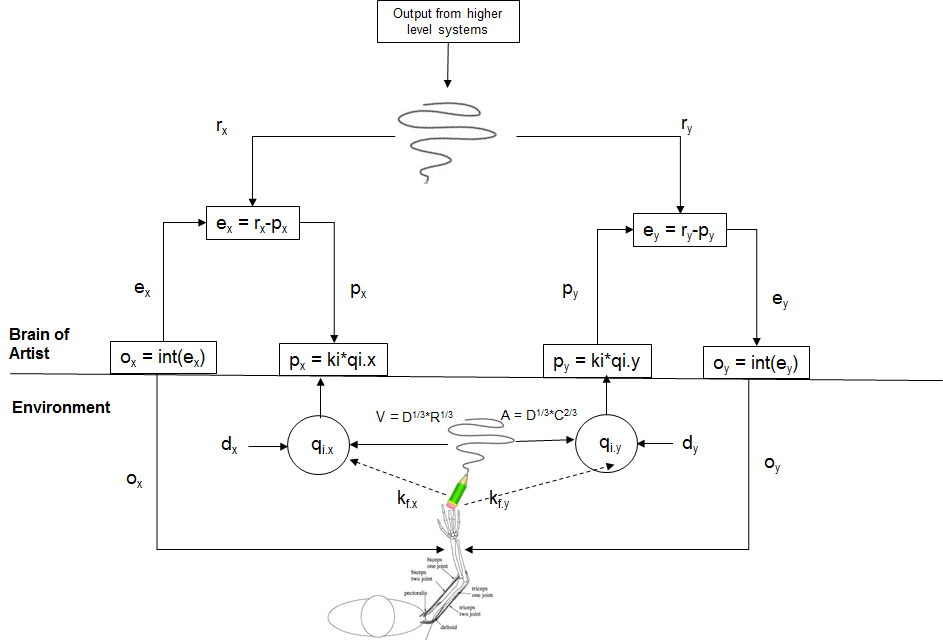
my first step was to develop a control model of someone
like an artist drawing a curved line. The model is
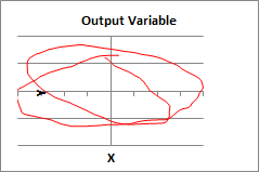
diagrammed below:
RM: The phenomenon to be accounted for by the model isthe curved pattern (squiggle) produced by the artist. The
completed squiggle is shown at the bottom of the figure,
in the environment where the squiggle is actually
produced. The model has to produce this squiggle exactly
as the artist produced it, by varying the position of the
pen over time. According to PCT, the observed variations
in pen position (qi.x and qi .y)
are controlled results of variations in the reference
specifications (r.x and r.y) for the perception of those
positions (p.x and p.y). Therefore the model varies these
references in a way that would produce the observed
variations in qi.x and qi.y.Â
RM: r.x and r.y are the references that you object to,claiming that they contain ad hoc temporal
dynamics. I question whether they do, but I agree that it
looks trivial (and a lot like cheating) to put the desired
end result (the squiggly movements of the qi .x
and qi .y over time) into the model (in the
form of the identical squiggly movements of r.x and r.y).
But that is the way the PCT model works; controlled
(intended) results are results that match specifications
set autonomously by the organism itself.Â
RM: But the reference signals in the control model arenot “cheating” any more than are the  “command” signals in
motor control models of behavior, like that of Gribble/Ostry ,
which is shown below. The commands in the model are
commands for output; forces that will produce movements of
the pen that will result in the observed squiggle. In the
PCT model, references, r.x and r.y, are commands for
input; perception that match the reference specifications.
RM:Â So both models have to use internal commands inorder to produce the observed result (squiggle). The
difference is that the commands in the PCT model “look
like” the observed result; the commands in the Gribble/Ostry
don’t necessarily “look like” the result produced. But in
both cases the commands have to be carefully crafted to
produce the correct result. So the possibility of
introducing “ad hoc temporal dynamics” is
present in both models. But the PCT model can do something
that the Gribble/Ostry cannot do: it can
control. That is, it can produce the intended squiggle in
the face of disturbances.Â
RM: Although the variations in the references (r.x, r.y) in the PCT model correspond to the squiggle that is
produced (qi.x, qi .y) , I
didn’t expect this simple model to produce a squiggle with
a power function relationship between angular velocity (V)
and curvature (R). I assumed, like you, that the power law
relationship was either 1) a controlled result in itself
(the person controlling for speeding up through tighter
turns), which would require a whole extra control
organization in the model or 2) the result of complex
dynamic characteristics of muscle force production (the
functions of e.x and e.y in the control model diagram
above) and/or of the feedback function connecting force
output to pen movement input (k.f in that diagram).Â
RM: So I was very surprised to find that the squiggleproduced by this simple control model showed a power
relationship between V and R . And when the squiggle was
an ellipse the coefficient of the power function was about
the same (~.31) as that found by Gribble/Ostry
for their ellipse production model  – a model with a far
more dynamically complex method of generating the ellipse
than my control model. That’s when I realized that the
observed relationship between V and R might be a
mathematical property of all curved lines. And, indeed, it
turns out that it is. The relationship between V and R,
which can be found using kindergarten math, isÂ
V= Â |dXd2Y-d2XdY|Â 1/3Â *R1/3Â Â Â
RM:  Note that the term  |dXd2Y-d2XdY |,
which I called D, implying that it was a constant, is a
variable. So the value of V for any curve is
proportional (exactly) to the 1/3 power of |dXd2Y-d2XdY |
and the 1/3 power of R.  I
was as surprised by this as as anyone. So I wanted to
make sure it was true so I did the multiple regression
analysis using log (Â |dXd2Y-d2XdY |
) and log (R) as predictors of log (V) for many
different “squiggles” and always found that all the
variance in log (V) was accounted for by an equation of
the form:
log(V) = .33* log (|dXd2Y-d2 XdY|) +.33*
log(R)Â
AGM:Second, you are stubbornly confused about the
difference between a mathematical relation
(that allows to re-express curvature as a function of
speed, plus another non-constant term that you insist
in ignoring and treating like a constant),
RM: I hope you see now that I do not treat thevariable  |dXd2Y-d2XdY |
 as a constant. The mathematical relationship is as
flawless as my kindergarten math teacher;)
Â
betweena physical realization (the fact that one can
in principle draw the same curved line at infinitely
different speeds),
RM: Actually, I understand that the same curved line(squiggle) can be produced at an infinity of different
speeds and by an infinity of different means (different
variations in o.x and o.y producing the same squiggle, qi .x,
qi .y). The same relationship between V and R
holds regardless of the speed with which the squiggle is
produced and and the means used to produce it. The
relationship between V and R is always:Â
log(V) = .33* log (|dXd2Y-d2 XdY|) +.33*
log(R)Â
RM: This samerelationship between V and R even holds for all the
different squiggly patterns made by o.x and o.y to
 produce the same squiggly pattern --qi.x, qi.y.Â
AGM:and between a biological fact (that out of all
possible combinations of speed and curvature, living
beings are, for yet some unknown reason —but therre are
tens if not hundreds of papers making proposals—
constrained following the power law,
RM: But now we know the reason. It's a result of thefact that the relationship between V and R for any curved
line is
V= Â |dXd2Y-d2XdY|Â 1/3Â *R1/3Â Â Â
RM:There is no way to draw a curved line so that this
equation does not hold. So there is no biological
constraint that creates the observed power law; it’s a
mathematical constraint.Â
RM: The reason peoplehave found different power coefficients for the
relationship between V and R is because they have left
the variable  |dXd2Y-d2XdY |  out
of the analysis. When you leave  |dXd2Y-d2XdY |  out
of the analysis, variations in that variable can lead
to different estimates of the power coefficient of R.
The amount by which the value of the power coefficient
of R is affected by leaving  |dXd2Y-d2XdY |  out
of the analysis depends on the shape of the squiggle
that  is
drawn. Leaving  |dXd2Y-d2 XdY| out of the
analysis of the V/R relationship for an ellipse
affects the actual power coefficient of R (.33) very
little, so the value obtained is around .31 (see
Gribble and Ostry, Table 1). Other squiggles can bring
the power coefficient of R down as low as .2.Â
RM:On that note, Martin Taylor noted that the power
coefficient for R, which is around .33 for a curved
figure drawn in the air, is closer to .25 when the same
figure is drawn  in a viscous medium (like water). It
turns out that this can be explained in terms of a
difference in the feedback function (k.f in the diagram)
in the two cases.Â
RM:In the PCT model, the feedback function is a simple,
linear coefficient. When the model traces out an ellipse
with a feedback function of k.f = 1.0, the power
coefficient of R is .32; when the feedback function is
changed to k.f = .5 – equivalent to trying to move a
pen through a more resistive medium – the power
coefficient of R is .26. This happens simply because the
ellipse drawn in the resistive medium is a little
sloppier than the one drawn in the air. The change in
feedback function changes the loop gain of the control
system.Â
AGM:But you will now reply for the n-th time saying that
everybody that has ever worked on the power-law miss es the point of control
systems and that your toy demo proves they don’t get
it.
RM: Yes. But they have been fooled by a ratherconvincing illusion. It’s hard not to see the observed
relationship between V and R as a situation where the
agent purposefully changes speed through curves (the power
law actually suggests that agents increase their speed as
the curve increases, but this increase in speed decreases
as curvature increases; it does not suggest that control
systems tend to slow down around sharp curves).
RM: So I agree that itis very surprising (and, perhaps, disappointing) that
the relationship between V and R tells us nothing about
how people draw curves. But that doesn’t mean that
research on how people (and other organisms) produce
curved paths should come to an end. To the contrary, it
opens up new and fruitful questions about exactly how
this is done. For example, the integral output function
that I use in the existing model is obviously an over
simplification. Something like the  Gribble/Ostry
model pictured above is probably a closed approximation.
A clever experimenter should be able to design
behavioral (and/or physiological) studies to determine
what the best model of the output function is.Â
RM:Going “up a level” (so to speak) research could also be
aimed at determining how what are presumably higher
level control systems set the references for the x,y
coordinates of the figure being drawn (assuming that the
figure is a controlled result and not a side effect of
controlling other variables, as in the CROWD demo).Â
RM:So there is really a lot of very important and
challenging research to be done in order to understand
how people draw figures. But this research must be based
on an understanding of the fact that the figure drawn is
a controlled variable – an intended result. And so any
research aimed at understanding how figures are drawn
must be based on an understanding of how control works.Â
AGM:But, again, ** you gloss over serious flaws
interpreting** the difference between mathematical
equations, physical conditions and biological
constraints as facts, ** and you magnify the
relevance of a toy demos** that, I wish could
shed new light, but so far don’t shed much new to the
problem.
RM: I hope this post helps. I don't believe I haveglossed over flaws. But if there are substantive flaws
please point them out. As I said above, if my analysis is
correct that doesn’t mean all is lost. Indeed, I think it
actually opens up many new and very productive
possibilities for research.Â
Best regards
Rick
SoI encourage you (and everyone still reading these
email exchanges) to say something new and relevant ,
because I still believe that asking what is being
perceived and what is being controlled is worth-while
in figuring out why speed and curvature are
constrained they way they are.
Â
Alex
–
Richard S. MarkenÂ
"The childhood of the humanrace is far from over. We
have a long way to go before
most people will understand that
what they do for
others is just as important to
their well-being as what they do
for
themselves." – William T. Powers