[Martin Taylor 2009.05.24.18.03]
[From Bill Powers (2009.05.24.0330 MDT)]
Martin Taylor 2009.05.23.23.56 –
At the end, you ask, “does this help?” The answer is,
“Were you trying to help, or just to scold me for not seeing what is
obvious to you?”
When I end a message, as I often do, with “Does this help” it is a
straightforward question. I want to know whether the message helped to
resolve an issue with which the person to whom I addressed the message
was struggling. The problem is that I can only guess the true nature of
the issue, and I hope that what I say does address it. I’m asking for
relevant feedback. I don’t believe I have ever used that phrase in any
other way, and nor do I intend to use it in any other way in the
future.
You were having problems understanding some questions, and I tried to
deduce how best to put the answers in a way that would help you
understand. I myself have a problem of understanding, in that I cannot
guess what I might have said that would lead to the annoyed tone of
your response.
From Bill Powers
(2009.05.23.11014 MDT)]
In Martin Taylor’s latest post, Martin Taylor 2009.05.23.14.18, he goes
through a nice clear development of the difference between two vectors,
with the two vectors each having as many dimensions as the number of
measurements of x or y in the original space.
That wording makes me wary of whether you did understand. Let me put
what
I said in another way. A vector is always of ONE dimension, no matter
how
many dimensions are in the space within which it lies. When you say
“vectors each having as many dimensions …” I am concerned
that you may think that the vector has more than one dimension. The N
components of a vector are the projections of the vector onto the N
axes
of the space, but that doesn’t change the dimensionality of the vector,
which is only one.
What I meant was that each of the components of the vector is in its
own
dimension orthogonal to all the others. The vector is the resultant of
all these individual vectors; it is inclined to each of the axes of
this
space by some angle. Since all the values of the component vector in
this
space are collinear in the original x-y space (aligned along one axis),
introducing this hyperspatial rendition seems irrelevant. You didn’t
explain its relevance.
He doesn’t quite get
to the
cosine bit, but next thing to it.
No, I had done that in the previous message [Martin Taylor
2009.05.22.15.45], to which the later one [Martin Taylor
2009.05.23.14.18] may be seen as a stage-setting foreword explaining
what
seemed not to have been clear in the earlier message.
You didn’t say that in the post. You may have thought it, but you
didn’t
say it.
I knew you had very recently read the earlier post on the cosine
question, and you asked about the point in the cosine message that
seemed to you to be problematic. That seemed to me to be sufficient
reason to expect that you would see the later message as explaining
issues that to you were problematic in the cosine message. I’m sorry if
it wasn’t so evident to you.
The difference between
the
vectors is a new vector whose length is computed by an “extended
Pythagorean theorem”, extending from the end of one N-dimensional
vector to the end of the other. It turns out that the difference
between
the two vectors is just SQRT(SUM((x[i] - y][i])^2)). However, that
quantity is relevant in a different discussion concerning tracking
errors
and prediction errors, and takes us away from correlations and
regression
lines.
No, it is critical in computing the correlation.
What, the difference between the vectors is critical? I thought the
correlation was obtained from the dot product of the two
vectors:
=============================================================================
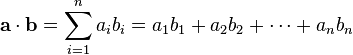
WIKI:
The dot product of two vectors
a = [a1, a2 , … ,
an] and b = [b1 ,
b2, … , bn]
is defined as:
 =============================================================================
Dividing that by the product of the vector lengths gives the
correlation.
I don’t see the difference between the two vectors in that.
So your insisting that the difference vector is critical to computing
the
correlation is not helpful, because as far as I can see, it isn’t
critical. What am I not understanding?
That when the triangle has three sides, and you are concerned with one
of the angles, the length of the opposite side is very important.
Here’s the original post [Martin Taylor 2009.05.22.15.45] again, or at
least the relevant bit of it, with the difference vector part
highlighted to show how it appears in the dot product. I hope the
boldface gets through the various mail systems.
Getting back to the unrelated issue of the relation between correlation
and the angle between two vectors, think of these same data as two
points in a 5-D hyperspace (there are 5 data pairs). The data set X is
represented by the point {0, 1, 3, 1.5, 4} (the order is important),
and Y is represented by the point {0, 3, 9, 4.5, 12}. The origin is, of
course, {0, 0, 0, 0, 0}. What is the angle between the vectors that
connect the origin to the two points?
If the sides of a triangle are a, b, c, and the opposite angles
are
alpha, beta, gamma, then cos(alpha) = ((b^2 + c^2) - a^2)/
(2bc). In
this case, alpha is the angle between the two vectors at the origin.
Their lengths are “b” and "c’, and the length of the difference
vector
is “a”. So,
b = sqrt(sum(xi^2)) = sqrt(0^2 + 1^2 + 3^2 + 1.5^2 + 4^2) = sqrt(28.25)
c = sqrt(sum(yi^2)) = sqrt(0^2 + 3^2 + 9^2 + 4.5^2 + 12^2) =
sqrt(254.25)
a = sqrt(sum(xi-yi)^2)) = sqrt((0-0)^2 + (1-3)^2 + (3-9)^2 +
(1.5-4.5)^2 + (4-12)^2) = sqrt(113)
So in this case, cos(alpha) = ((sum(xi^2) + sum(yi^2) -
sum((xi-yi)^2))/2(sqrt(sum(xi^2)sum(yi^2)) = (28.25 + 254.25 -
113)/2sqrt(28.25254.25) = 169.5/169.5 = 1.0 (The notation in straight
ASCII is visually a bit cumbersome, but I hope you understand what it
means).
The formula can be simplified, since __sum(xi-yi)^2 = sum(xi^2) +
sum(yi^2) - 2sum(xiyi)__, which makes the numerator become simply
__2sum(xiyi)__. The formula is then
cos(alpha) = __sum(xiyi)__/sqrt(sum(xi^2)*sum(yi^2))
That is exactly the Wikipedia formula. Sum(xi-yi)^2 is the square
of the length of the difference vector.
It seems to me that
the angle
whose cosine is r not observable. To observe it we would would have to
be
able to perceive a plane surface in N dimensions and see a triangle
drawn
in that plane, which I can’t imagine.
I accept that you can’t imagine it, but I can’t imagine why you can’t.
That is not helpful, either. I can’t see that triangle tilted relative
to
the multiple axes of this space. I can imagine seeing a triangle
face-on,
but from what direction in the multiple-dimensioned space would I have
have to be looking to see it that way? You claim you can see it, and if
that’s true I congratulate you, but unless you can tell me how to do
that, I don’t get much advantage from your ability to do so.
I don’t suppose it will be helpful to repeat my mantra that a triangle
is just a triangle, and once you have established the side lengths, you
really aren’t concerned any more with the hyperspace, at least not when
you are considering the relations among the variables, because the
hyperspace representation is of the full ordered data set and you don’t
care about that any more. I can’t imagine seeing the triangle in (for
the tracking triangulations) 3600-D space, but I can imagine seeing the
shape of the triangle, whether it is needle-pointed, near equilateral,
right-angled, or whatever. That’s all you want, once you have used the
N-dimensional locations of the vertices to establish the side lengths.
A triangle is just a
triangle.
It has vertices A, B, C, sides of length a, b, c, and angles alpha,
beta,
and gamma. All nine of those parameters are simple real numbers. I’ll
repeat my mantra: you are trying to see difficulty where simplicity
exists.
But a triangle also has orientations – eight axes of rotation in an
8-dimensional space, for example – as well as a location, another
eight
measures. Why are you ignoring those aspects of the triangle? If I
understood that, I would be happy to ignore them, too – but I
don’t.
Ah, maybe I begin to see your difficulty at last. (But maybe not. I
hope I do).
Let’s get at the answer by stages. We look first at a different issue.
What are those 8 axes? What does a triangle vertex actually represent?
To answer those questions, let’s get at it a little obliquely, and
suppose that the 8 measures of x and y are 8 samples in a time-sequence
of samples, {x1, y1} taken at t1, and so forth. The eight values of x
are {x1, x2, x3, …x8}. I’ll describe four different ways of
representing those data.
-
You could draw the x values as a sampled waveform on a graph with a
time axis for the abscissa and x1, x2, x3… x8 as the successive
ordinate values. On this same graph, you could draw another waveform
for {y1, y2, y3,…y8}. You would have two curves on one graph, and to
show the relations between them, you might look to see whether they
both go up and down at the same times. The graph represents the
complete data set, including its ordering.
-
There’s another way of looking at these same data, which is to have
a 3-D graph, on which left-right is a time axis, up-down is x value,
and front-back is y-value. In this 3-D plot, there is one point at time
t1, with the up-down coordinate x1 and the front-back coordinate y1.
There’s another point for time t2, another for t3, … t8. Now we can
take those points and draw a curve through them in 3-D space. This
simple curve has all the same information as did the two curves in the
2-D graph. You see how well x and y are related by looking to see
whether the curve tends to lie near a diagonal plane, as it will if,
say, y = ax + b + noise.
-
Here’s a third way of viewing the same data, the one you find most
congenial. Collapse representation 2 along the time axis, leaving only
the up-down and front-back axes to define a graph on which all the
corresponding x, y pairs are plotted, each y against its corresponding
x. We call that a scatter-plot, and it loses the time information,
since there’s nothing in the graph to show whether THIS point or THAT
one represents data taken at time t1, t6, or t8. You could, of course,
label them or even connect the dots with a loopy curve in the order the
data were taken, but one usually doesn’t do this. The scatter is
sufficient for the purpose of estimating correlation visually. This
representation keeps the relative vales of xn and yn measured at tn,
but loses the ordering of the data pairs, which you don’t need in order
to compute correlation.
-
Now we introduce a fourth way of showing the data – well, not
actually “showing”, since one can’t represent a high-dimensional space
on paper. We keep the time information as we did in the first two
cases, but instead of laying the time out on a line, we use it to label
the axes of a space. Think first of a sequence of only three samples of
x and y, taken at t1, t2, and t3. Plot the three x values so that the
coordinate of the t1 value is left-right, the t2 value is up-down, and
the t3 value is front-back. Now there is a point at {x1, x2, x3}.
There’s only one point, but it represents the whole ordered time series
of x values. The location of the point describes a time series of three
values, just as in representation 2 each point represented not an
x-value or a y-value, but an x-y pair of values.
4 (cont). In the 3-D space representing a time series of three samples,
we can also place a point that represents the waveform of y, y1 being
its coordinate on the left-right axis, y2 its coordinate on the up-down
axis, and y3 its coordinate on the front-back axis. Now comes the
interesting part. How does correlation between the x and y waveforms
show up in this representation, which incorporates all the temporal
information in the same way as did method 2? High correlation means
that when x is high, so is y, proportionately, and when x is low, so is
y, proportionately. Accordingly, if x and y are perfectly correlated,
and any constant difference between them has been eliminated, the
points for the origin, for x, and for y will be colinear. If there is
noise in the measurements, or if there isn’t a real linear functional
relation between them, the point that represents the y waveform will be
in a different direction from the origin than the point that represents
the x waveform. There will be a non-zero angle between the vectors from
the origin to the x-point and the y-point. In fact, as the calculations
in other messages have shown, the cosine of the angle between them is
their correlation.
4 (cont). Now we are getting near the answer to your question. Let’s
augment the time sequence so that we have 8 x-y pairs taken at times
t1, t2, …, t8. We can make a representation that extends the 3-D
space to 8-D. In this space we have one point that represents the
entire x waveform. Its coordinates are {x1, x2, x3,…x8}. We have
another point that represents the y waveform, remembering that axis 1
still represents the value at t1, axis 2 represents the value at t2,
and so forth. One can define a vector from the origin to each of these
two points, the one represnting the x time series and the one
representing the y time series. One can’t visualize as a picture in
one’s mind how a vector is oriented in the 8-D space, but since
notionally it’s just a straight line, that may not matter (and it turns
out that it does not matter). Just as in the 3-D space of 3
time-samples, if the variation in the y waveform is simply proportional
to the variation in the x waveform, the vector for y will be in the
same direction from the origin as the vector for x.
4( cont). Now think back to the relation between representations 2 and
3 above. Representation 3, the scatter plot that loses time sequence
information, is enough to show you the correlation between x and y, as
also is representation 2, the 3-D time-series graph. In fact, because
representation 3 eliminates the time variable, the correlation is
easier to see than it is in representation 2. What does the orientation
of the vector from the origin to the x-point represent? It is the time
sequence of the data. If you rotate the x-vector in the space, you
change the x-values at the different sample times. If you relabel the 8
axes, you change the ordering of the samples. Relabelling doesn’t
present a problem, because the same reordering will happen for x and
for y, so their covariation will not change. It’s less easy to show
that rotating the space doesn’t affect the relationship between x and
y, because rotating actually changes the sample values represented.
However, your question, which now is nearly answered, is why this
doesn’t matter.
4 (cont) What we are interested in is the correlation between x and y.
Previously, it has been shown that this correlation is exactly the
cosine of the angle between the x and y vectors in the space. Many
different series of values lead to the same correlation. Rotating the
two vectors in the space while keeping their relative angle constant
changes the locations of the points representing x and y. These
different locations represent quite different time series, but since we
are keeping the angle constant between the x-vector and the y-vector
when doing our rotations, the two new time series will have the same
correlation as the original x and y time-series. Since they have the
same correlation, and we are not trying to recover the actual time
series from the calculation of the angle, we can orient the triangle
how we choose. We can lay it down on the 1-2 plane if we want, or we
can imagine it where we will. It makes no difference to the
correlation, provided we maintain the shape of the triangle.
The end result of all this is that you have to worry about the triangle
orientation only if you need to keep track of the actual data samples
and their sequence, which is not the case when you are computing a
correlation. When computing the correlation, you need only to be
concerned with the lengths of the three sides of the triangle, which
suffice to define each angle of the triangle.
I hope that all makes sense, and that it covers the issues raised in
the following parts of your message.
Now I return to my
exploration
of my misunderstandings.
I said that Rick says
r = z.y/z.x
That can’t be right because z.x, z.y is only a single point.
As I understood Rick, it means that for a particular x value, you can
find the corresponding (expected) y value from the equation z.y = r *
z.x. It’s not intended to get r from a single x or y
value.
But you can solve that algebraic expression for r:
r = z.y/z.x
That can’t possibly give the correct value of r, since z.y/z.x is not
the
same for every data point.
Correct. If I understood Rick correctly, r is given. You aren’t
supposed to be deriving it from the values of one point, but rather,
you are supposed to be estimating an as yet unmeasured y, knowing its
corresponding x. How well that will actually represent y when it is
later measured depends on the correlation (though of course, you could
get lucky with any value of correlation, even zero!).
I ask seriously: did this help?
Martin
 =============================================================================