Behavioral Illusions: The Basis of a Scientific Revolution

[rsmarken]

Hi Adam

RM: As you know, I forgot everything I knew about PCT when Bill passed away (indeed, became the enemy of PCT by some accounts)

AM: You did not forget, you never really knew the mathematical aspects of control theory, from what I can see in the archives and from what you are writing now. Bill spent some 30-40 years before you met him
working with analog computers and designing control systems.
You never went down that path, so while Bill was alive, he would nicely and patiently correct you and direct you with the more difficult parts of the math.
It would do you good to study classical control theory, maybe from an old textbook. It seems process control has similar terminology to PCT, maybe that would be a good start.

RM: A deep knowledge of classical control theory is not necessary in order to understand PCT. Indeed, it can get in the way. Early in the life of CSGNet we had a control engineer take an interest in PCT and he couldn’t (or wouldn’t) get it at all. I think Bill’s attempt to get the guy to “get” PCT is somewhere in the archives. You seem to be able to go through those pretty well so I’ll let you find it. It’s probably from 1990.

RM: And I was in on the discussions between Bill and John Flach, a psychologist who knows the mathematics of control theory far better than Bill did – Bill struggled to learn Laplace transforms to try to keep up with him – and all that math didn’t help him get PCT; indeed, the interaction led to the work shown in the “adaptation without adaptation” chapter of LCSIII – work that Flach didn’t get at all.

RM: And i don’t remember Bill patiently correcting and directing me with the more difficult parts of the math. But if he did it wasn’t often and that’s the kind of correction that was particularly useful. The things people don’t get about PCT are not related to the math, they are about how the model maps to behavior. That’s why Bill was unable to get many (any?) experts in classical control theory to understand how control theory should be applied to behavior.

RM: And when it comes to Bill correcting people on the net, I think you should take a look at his posts to others besides me. As I recall, Bill’s main complaints about me were about my tone, not about my understanding of PCT. If you want to see Bill complaining about people’s understanding of PCT – people who now claim to be experts in PCT – you might take a look at Bill’s posts to Martin Taylor regarding Martin’s ideas about there being “information in perception about the disturbance”, or about his belief in affordances or about there being an entity called a CEV.

RM: But I’m tired of the insults and the condescending comments from you. And I really don’t want to do this on my own anymore. I used to have Bill but now there is no one – at least no one on this net – who is willing or able to take my “side” of this argument. So I’ll leave at least for a while and let you carry on as you wish. But while you’re telling people how little Bill thought of my understanding of PCT you might point them to Bill’s preface to MIND READINGS to see what Bill said he thought of my work. Of course, that’s probably Fake News, right?

Best

Rick

[amatic]

You get terribly dramatic when it comes to you being wrong.

First I was the Spanish inquisition, forcing you Mr. Galilei to admit falsehoods. Now I’m Trump slapping and you, the honest FBI agent, for doing his job. You are dramatically leaving the scene, head bowed down. Someone yells “You are a poster child for the Dunning-Krugger effect!”. You turn around, eyes closed, showing your tongue, and exit.

I think you are leaving because you cannot face the fact that you could be wrong. That would mean that, horror of horrors, Martin Taylor was right! Alex was right for calling bullshit! Everyone else on the net who disagrees with you on the topic of the power law was right, and you were really the enemy of PCT.

It probably is not easy to deal with those possibilities, but you made your own bed.

RM: The observed relationship between monthly ice cream sales and murder rate. And all other spurious correlations, like that between curvature and velocity of movement.

A spurious correlation is not a statistical artifact. Ice cream sales and murder rates can be really correlated in some cases. The correlation is spurious because they are not causally related.

Instantaneous curvature and velocity are also correlated in some cases and are not causally related. No one ever said they were causally related, you have misread or misunderstood that. Stretching the definition, you could say that it is a spurious correlation, if you would show the real mechanism producing the correlation, and all the causal factors - the controlled variables, input and functions, etc.

A statistical artifact, by definition, is not a real phenomenon. The correlation itself is not reflecting a real correlation. Empirically, fast hand movement in elliptical trajectories shows a real correlation between speed and curvature, as many people have been showing for many years. I’ve also put up here a little plot of speed and curvature, color coded, that shows how people move slower in the curved parts, and faster in the flat parts. You said you can see that, yes, people do really move slower in the more curved parts.

You’ve confused two terms in statistics, a spurious correlation and a statistical artifact. What does that say about your knowledge of statistics?

There are statistical problems with power laws, but the fundamental problem of the speed-curvature power law is - why do people move slower in curved parts? Empirically, before any statistics, you can see it in the plots, they do move slower in the curved parts, if the average velocity is high enough. That is what all the “power law people” are studying. What are the mechanisms of tracing lines, of drawing letters, of making rhythmical hand movements, etc. Whatever the mechanisms is, it has to slow down in curved parts, and go faster in the other ones.

The perspective of PCT is to search for perceptual variables that are maintained, and the control loop that produces the slowing down as a side effect.

AM: Well, that is your theory then. You prefer to call it a hypothesis? The speed-curvature power law is a statistical artifact that results from the failure to include the variable D in the regression.

RM: I’s neither a theory nor a hypothesis; it is a mathematical fact.

Calling some phenomenon a statistical artifact is an interpretation, a hypothesis, not a fact. The equation you mention is a mathematical fact, but different people have different interpretations of that equation, so that is the debatable part.

RM: What I and apparently everyone else who studies the power law knows is that the mathematical relationship between the measures of curvature (R or C) and speed (V or A) used in these analysis is a power law relationship of the form:
RM: log (V) = 1/3* log( R) + 1/3* log(D)

That is a correct equation. If you rearrange the equation, you get D = V^3 / R. What you have done is discovered a formula for calculating D from speed and the radius of curvature and rearranged it. If you further rearrange it and play with algebra, you would get that D = | a x v |.

The jump you make between this formula and calling the empirically found correlation a statistical artifact is the problematic part.

RM: this because the 1/3 and 2/3 power law are right there in the mathematical equations relating the variables they use to measure speed and curvature .

This part.

The power law is not in the mathematical equations relating speed and curvature. It is in the equation relating speed, curvature and affine velocity. There is a big difference.

A mathematical equation that relates speed and curvature would have to have just speed and curvature in. V = f( C ). This is not the case. Speed and curvature are not related mathematically, they can vary independently, just like you can drive your car faster or slower in the curves, or draw lines with any speed you please (if it is slow enough). In principle, a particle can move with any speed trough any curvature. And still, the formula you mentioned would be valid, because that is just a formula for calculating affine velocity from speed and curvature.

[amatic]

RM: A deep knowledge of classical control theory is not necessary in order to understand PCT.

Oh, I’m not saying you don’t have a deep knowledge of classical control theory. I’m saying you don’t have the BASIC knowledge of classical control theory, and the math that is needed to understand the behavioral illusion. If it makes you happy, it looks like that neither Martin Taylor had it.

Not fake news, here is Bill correcting you two bozos on how to derive the equations of the behavioral illusion in 2010! [Beyond the Fringe (was An Opportunity for PCT PR) - #26 by Bill_Powers1]

That is just a small example. In the previous topic on the behavioral illusion, where I followed the 1978 paper derivation, you made the same kinds of mistakes, just like in this topic.

[amatic]

You made exactly the same type of error in the previous topic where you wrote that qi is related by the feedback function to qo. This would imply qi = f(qo), which is not true. qi = f1(qd) + f2(qo).

Now you are saying that because R = V^3 / D, speed is related to radius of curvature. Again not true, because the term “related” implies that V = f ( R ). All that formula says is that if you had any the two variables calculated or measured, you could find the third one.

RM: I used to have Bill but now there is no one – at least no one on this net – who is willing or able to take my “side” of this argument

You have no one on your side because you are wrong. In your papers on the power law and behavioral illusion, as I’ve demonstrated, you’ve been wrong on the definition of the behavioral illusion. You’ve been wrong on the issue of side effects reflecting properties of the control loop. Now you incorrectly defined the term statistical artifact. And those are just the terms in the TITLE of your papers. You are also wrong about speed and curvature being mathematically related.

Bill would have been deep on the opposite side of the power law argument, and he would have cut it long before you could publish a paper. For the derivation of the behavioral illusion equations, Bill gave you a B. For this nonsense with the power law, you’d be flunked back to high school.

Here is what Bill said about one “power law experiment” : [From Bill Powers (930428.0700)]

“In JEP-Human Perception and Performance, there was a good control-theory experiment:
Viviani, P. and Stucchi, N. Behavioral movements look uniform: evidence of perceptual-motor interactions (JEP-HPP 18 #3, 603-623 (August 1992). Here the authors presented subjects with spots of light moving in ellipses and “scribbles” on a PC screen, and had them press the “>” or “<” key to make the motion look uniform (as many trials as needed). The key altered an exponent in a theoretical expression used to relate tangential velocity to radius of curvature in the model. The correlation of the formula with an exponent of 2/3 (used as a generative model) with the subjects’ adjustments of the exponent was 0.896, slope = 0.336, intercept 0.090. This is just the kind of experiment a PCTer would do to explore hypotheses about what a subject is perceiving. By giving the subject control over the perception in a specified dimension, the experiment allows the subject to bring the perception to a specified state – here, uniformity of motion – and thus reveals a possible controlled variable (at the “transition” level?). The authors didn’t explain what they were doing in that way, but this is clearly a good PCT experiment. Even the correlation was respectable, if not outstanding (the formula was rather arbitrary, so it should be possible to improve the correlation considerably by looking carefully at the way the formula misrepresented the data).
There is a world of difference between the kinds of experiments reported in J Exp. Soc. Psych and the two described above (and between the two described above and most of the others in JEP).”

AM: So, there is a dot moving on the screen, according to a speed-curvature power law with an adjustable exponent. Meaning - subjects adjust the amount of slowing down in the curves. The idea is to see which exponent results in the perception of uniform motion. There are no issues of “speed and curvature being related” for that particle. Instead of a particle, put someone’s hand moving according to the same equation. No difference in the math. “This is just the kind of experiment a PCTer would do”.

It is not everyone else, it is you.

[rsmarken]

Hi Adam

RM: I’ll reply to this because I think it is relevant to my point of view on power law research:

AM: Here is what Bill said about one “power law experiment” : [From Bill Powers (930428.0700)]

BP: “In JEP-Human Perception and Performance, there was a good control-theory experiment:
Viviani, P. and Stucchi, N. Behavioral movements look uniform: evidence of perceptual-motor interactions (JEP-HPP 18 #3, 603-623 (August 1992). Here the authors presented subjects with spots of light moving in ellipses and “scribbles” on a PC screen, and had them press the “>” or “<” key to make the motion look uniform (as many trials as needed). The key altered an exponent in a theoretical expression used to relate tangential velocity to radius of curvature in the model. The correlation of the formula with an exponent of 2/3 (used as a generative model) with the subjects’ adjustments of the exponent was 0.896, slope = 0.336, intercept 0.090. This is just the kind of experiment a PCTer would do to explore hypotheses about what a subject is perceiving. By giving the subject control over the perception in a specified dimension, the experiment allows the subject to bring the perception to a specified state – here, uniformity of motion – and thus reveals a possible controlled variable (at the “transition” level?). The authors didn’t explain what they were doing in that way, but this is clearly a good PCT experiment. Even the correlation was respectable, if not outstanding (the formula was rather arbitrary, so it should be possible to improve the correlation considerably by looking carefully at the way the formula misrepresented the data).
There is a world of difference between the kinds of experiments reported in J Exp. Soc. Psych and the two described above (and between the two described above and most of the others in JEP).”

RM: Yes, I know about the Viviani & Stucchi (1992) experiment and, in an effort to end our M&S 2018 reply on a positive note, I referred to it as an example of the kind of experiment one might do to study control of movement. Bill found this paper in April 1993, while searching through current issues of various psychology journals for examples of psychological research that looked like they didn’t need to be “deposited in the wastebasket” (the phrase he used in his Foreword to MIND READINGS to describe what the work described in that book suggested should be done with “a whole segment of the scientific literature”).

RM: Bill found the Viviani/Stucchi paper in JEP: HPP and saw that it looked like a good control theory experiment. Indeed, it looks a lot like a test for the controlled variable. It was different than most other conventional experiments because the researchers seemed to be aware of the fact that producing a motor movement (like moving the finger around in an elliptical or squiggly trajectory) was equivalent to producing a perception (in this case, of a spot of light moving around in an elliptical or squiggly trajectory). The hypotheses in the experiment was like a hypothesis in the TCV: that the the perception (and, presumably, production) involved control of a perception of a power relationship between curvature and velocity that had a coefficient – beta – was close to .33. The “disturbance” to this movement was the initial setting of beta that was ,. to .33 and the subject could compensate for this disturbance by pressing the > or < keys to increase of decrease beta.

RM: The results impressed Bill because he seems to have found a high correlation (.896) “of the formula with an exponent of 2/3 [did he mean 1/3?] with the subjects’ adjustments of the exponent”. I couldn’t find that correlation reported in the paper and his description of it makes no sense to me. But he certainly wasn’t impressed by the research because of the assumption of a power law relationship between curvature and velocity with a particular exponent. You can see this in the quote above where Bill says that “…the formula [used to generate spot movement] was rather arbitrary, so it should be possible to improve the correlation considerably by looking carefully at the way the formula misrepresented the data”. I think that can be interpreted as saying that the hypothesis that a 2/3 (or 1/3) power relationship between speed and curvature is what is being controlled when controlling for uniform movement should be rejected and a new hypothesis tested.

RM: So while the Viviani/Stucchi study is as good an example of a PCT- like study as one is likely to find in the conventional literature, it could be considerably improved if carried out with an understanding of how control works in living systems. So this study would be a great place for power law researchers to start developing research aimed at understanding the perceptual variable(s) involved in the control of movement. As I said in the conclusion to M&S 2018:

… once the controlled perceptual input variable is identified it should be possible to build a simple control system model that explains the movement behavior produced by living systems as it occurs under many different circumstances, as was the case with our object interception model noted above. To paraphrase Powers’ conclusion to his 1978 Psychological Review paper (p. 434): for a thousand unconnected empirical generalizations about movement behavior that are based on superficial similarities between features of movement trajectories, we here substitute one general underlying principle: control of input.

Best regards

Rick

[amatic]

The point is, Bill was working in an observatory. He knew all about orbital mechanics, power laws, speeds, angular speeds, curvatures, etc. He saw nothing wrong mathematically with a point on a screen moving in an elliptic trajectory, having different amounts of slowing down in the curved parts, and having this motion described by a power law.

If you want to generate a power-law path, you simply calculate the speed to be the cube root of curvature or whatever, and keep staying on the path. Nothing to it for a computer.

You, on the other hand, claim that “curvature and speed are mathematically related”, which is utter nonsense; does not come out of the formula for calculating D, and Bill would have caught the error right in the beginning.

[rsmarken]

Hi Adam

AM: The point is, Bill was working in an observatory. He knew all about orbital mechanics, power laws, speeds, angular speeds, curvatures, etc. He saw nothing wrong mathematically with a point on a screen moving in an elliptic trajectory, having different amounts of slowing down in the curved parts, and having this motion described by a power law.

RM: Nor do I. But that’s irrelevant to why Bill thought the Viviani/Stucchi experiment was like a control theory experiment. It was like a control theory experiment because… actually, why don’t you tell me why Bill thought it was like a control theory experiment.

AM: If you want to generate a power-law path, you simply calculate the speed to be the cube root of curvature or whatever, and keep staying on the path. Nothing to it for a computer.

RM: Even more nothing nowadays with computers that are nearly 30 years newer. Could you send me the computer algorithm they used to generate the spot movement? I’d like to see what they look like.

AM: You, on the other hand, claim that “curvature and speed are mathematically related”, which is utter nonsense;

RM: And yet they are mathematically related: V = R^1/3 * D^1/3 and A = C^2/3 * D^1/3. There is a no-nonsense, mathematical (power) relationship between speed (V, A) and curvature (R, C).

AM: does not come out of the formula for calculating D, and Bill would have caught the error right in the beginning.

RM: There is no error. If you use regression analysis to analyze the spot trajectories used by Viviani and Stucchi I think you will find the beta value they used to generate each one if you just regressed R on V or C on A. But if you include D in the regression you would find that the power coefficient (beta) of R regressed on C to be exactly 1/3 and the power coefficient of C regressed on A to be exactly 2/3 with R^2 values of 1.0 for both regressions. At least I’m pretty sure that that’s what you would find. Try it and see. Or I’ll try it if you like; just send me the Viviani/Stucchi algorithm for generating the spot trajectories.

RM: But, again, Bill’s evaluation of the Viviani/Stucchi experiment as being like a control theory experiment had nothing to do with how the spot movements were produced or whether the algorithm that produced them was based on a power law formula (remember, Bill did say that “the formula [used to generate spot movement] was rather arbitrary”). Bill saw the Viviani/Stucchi experiment as control theory-like for reasons that had nothing to do with the power “law”. If you can figure out what that reason was you may be on your way to becoming a researcher who knows the proper way to study the behavior of living control systems.

Best

Rick

[amatic]

Here is some python code for generating a trajectory with angular velocity equal to curvature raised to arbitrary exponent, with possibility to average speed or total time.

def get_times(ds, C, target_time, target_beta):
  dt = ds * C ** (1- target_beta)
  T = cumsum(dt)
  k = target_time / T[-1]
  t =  k * T 
  return t

def retrack(x, y, t, target_beta, target_time=None):
  if (target_time == None): target_time = t[-1]
  r = analyze(x, y, t) # get arc-length ds and curvature C
  ts = get_times(r.ds, r.C, target_time, target_beta)  # get target power law exponent, and target duration
  d = analyze(r.x, r.y, ts) # using new time vector, resample to const dt
  return d

rest of the code: Google Colab

In short, you take the time variable of an arbitrary trajectory, then set the time between each to points such that speed equals the desired value. Then resample the whole trajectory into equally spaced time intervales.

RM: Nor do I. But that’s irrelevant to why Bill thought the Viviani/Stucchi experiment was like a control experiment.

Uniformity of movement as a potential controlled variable. Now, back to bold. It is very relevant to the topic of the power law that you don’t see the problem that a dot of light is moving according to a power law, and yet you do see a problem when a human hand is moving, approximately, according to the same formula.

Why is that? The formulas don’t know what made the trajectory, if it was generated by a computer or by a human.

RM: And yet they are mathematically related: V = R^1/3 * D^1/3 and A = C^2/3 * D^1/3. There is a no-nonsense, mathematical (power) relationship between speed (V, A) and curvature (R, C).

The exact analogy of this is saying that two sides of a right triangle are mathematically related. If you have sides a and b closing the right angle, and the side c as the hypothenuse, Pythagoras’ theorem is not relating two of the sides, it is relating three of them. c² = a² + b². Any two sides are not mathematically related, and neither are speed and curvature. Instead, speed, curvature and D are related, and we have time as the additional variable. If you look at the code above, you can see something like:

V = sqrt(xvel**2.0 + yvel**2.0)
D = abs(yacc * xvel - xacc * yvel)
R = (V**3.0) / D

Written in that order (in function analyze). First, calculate speed from x and y components of velocity (xvel, yvel). Then calculate D as a cross-product of acceleration (xacc, yacc) and velocity (xvel, yvel). Then calculate radius of curvature according to the formula you mention. These are all lists of scalar values, with time as the fourth implicit variable.

RM: There is no error. If you use regression analysis to analyze the spot trajectories used by Viviani and Stucchi I think you will find the beta value they used to generate each one if you just regressed R on V or C on A. But if you include D in the regression you would find that the power coefficient (beta) of R regressed on C to be exactly 1/3 and the power coefficient of C regressed on A to be exactly 2/3 with R^2 values of 1.0 for both regressions. At least I’m pretty sure that that’s what you would find. Try it and see. Or I’ll try it if you like; just send me the Viviani/Stucchi algorithm for generating the spot trajectories.

There is no error in the raw calculating process. For any trajectory, given your procedure, I get the same results. No problem there. I have the issue with your interpretation of that procedure.

Should the omitted variable bias improve the prediction of the criterion variables from the predictors and the regression parameters?

RM: If you can figure out what that reason was you may be on your way to becoming a researcher who knows the proper way to study the behavior of living control systems.

That is condescending. You are implying that you know the proper way to study them, and that you can judge whether I know it. Now I could call you Master Marken, or whatever, to mock the implication, but that doesn’t really lead us anywhere.

[amatic]

Here is an illustration of the error of claiming that two variables are mathematically related, while in the formula there are three variables.

link to code

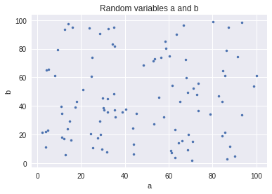
Variables a and b are lists of 100 items, completely random scalar values, in the range of 0 to 100, generated by this code:

a = np.random.random(100) * 100 
b = np.random.random(100) * 100

The correlation between them is near zero, and so is the r2. There is no statistical procedure that will make them mathematically related.

Now I introduce a third variable c with the following code:

c = 3 * a + 0.5 * b

Then I use linear regression with predictors a, and c, and criterion variable b.
regr.fit( df[['a', 'c']], df["b"])

This gives me back coefficients -6 and 2 for the predictor variables, which is exactly the formula for c rearranged, b = -6a + 2c. I get the same result for any list of random variables a and b. I also get the correct coefficients in all the cases I’ve tested.

This did not make a and b mathematically related. They are still completely random variables, and simply introducing a formula to calculate c does not change the randomness and does not create a mathematical relationship between a and b.

The same procedure, without fail, always returns the coefficient 0.33 for the ellipse speed, radius of curvature and D. The formula R = V^3 / D does not make speed and radius of curvature mathematically related.

[rsmarken]

Hi Adam

@amatic

AM: Here is some python code for generating a trajectory with angular velocity equal to curvature raised to arbitrary exponent, with possibility to average speed or total time.

def get_times(ds, C, target_time, target_beta):
  dt = ds * C ** (1- target_beta)
  T = cumsum(dt)
  k = target_time / T[-1]
  t =  k * T 
  return t

def retrack(x, y, t, target_beta, target_time=None):
  if (target_time == None): target_time = t[-1]
  r = analyze(x, y, t) # get arc-length ds and curvature C
  ts = get_times(r.ds, r.C, target_time, target_beta)  # get target power law exponent, and target duration
  d = analyze(r.x, r.y, ts) # using new time vector, resample to const dt
  return d

RM: I’m afraid I don’t read Python and I’d rather not take the time to learn right now. Could you just give me some relatively simple pseudocode that will vary the x,y coordinates of a spot moving in a squiggle pattern over time according to a power law; V = R^1/3 or A = C^1/3 into the time? Or better yet could you just send me several columns of x,y coordinates of a spot moving in a squiggle pattern according to a power law with several different beta values? Or even better still would be both. I would like to see what the movement looks like with different coefficients and do the regression analysis on the trajectories.

RM: Nor do I. But that’s irrelevant to why Bill thought the Viviani/Stucchi experiment was like a control experiment.

AM: Uniformity of movement as a potential controlled variable.

RM: I would say they were testing to see what variable is being controlled when a person is controlling a perception of uniform motion. Their hypothesis was that subjects control the value of beta in a power law equation relating speed to curvature. The assumption was that subjects would see uniform movement (which I presume means constant speed movement) when beta is .33. The disturbance to the hypothetical controlled variable was the initial setting of beta. Subjects corrected for this disturbance (if they needed to) and brought their perception of the movement back to the reference state of “uniform”, by pressing the “>” or “<” keys, in order to get beta = .33.

AM: Now, back to bold. It is very relevant to the topic of the power law that you don’t see the problem that a dot of light is moving according to a power law, and yet you do see a problem when a human hand is moving, approximately, according to the same formula.

AM: Why is that? The formulas don’t know what made the trajectory, if it was generated by a computer or by a human.

RM: The power law has nothing to do with why the Viviani/Stucchi study makes sense from a control theory perspective and other power law studies don’t. The Viviani/Stucchi study actually tests for a controlled variable; other power law studies don’t. The fact that the hypothesized controlled variable in the Viviani/Stucchi study is a power coefficient is beside the point. At least it is treated as a hypothesis about a variable aspect of the movement that might be controlled. Power law studies just look at features of the movement itself under the assumption that this will tell them something about how the movement is produced; it won’t.

RM: And yet they are mathematically related: V = R^1/3 * D^1/3 and A = C^2/3 * D^1/3. There is a no-nonsense, mathematical (power) relationship between speed (V, A) and curvature (R, C).

:AM: The exact analogy of this is saying that two sides of a right triangle are mathematically related.

RM: It just struck me as a pretty amazing coincidence that in the equations above the power exponents of R and C --1/3 and 2/3, respectively – are exactly the exponents that have been proposed as those that characterize the power “law”; a law that, I believe, is presumed to reflect properties of nature (behavior), not of mathematics. Indeed, in many articles on the power law the title often says that the article is about the “1/3 power law” or the “2/3 power law”.

AM: Should the omitted variable bias improve the prediction of the criterion variables from the predictors and the regression parameters?

RM: Yes, unless all of the variance in the criterion variable (V or A) is accounted for by the included predictor (R or C). This would be the case, for example, in a perfect ellipse, which follows the power “law” exactly.

RM: If you can figure out what that reason was you may be on your way to becoming a researcher who knows the proper way to study the behavior of living control systems.

AM: That is condescending.

RM: You are absolutely right and I apologize. I didn’t intend it to be condescending but I should have known that it might be taken that way. Civil behavior is all about knowing what the unintended consequences of one’s behavior might be and trying to avoid them. So I am sorry.

I would really appreciate it if you could get that data that I asked for to me, if possible – the time varying x.y coordinates of the Viviant/Stucchi power law generated spot squiggle movements. And the pseudocode too?

Best

Rick

[amatic]

RM: Or better yet could you just send me several columns of x,y coordinates of a spot moving in a squiggle pattern according to a power law with several different beta values?

Here is an excel file with the squiggles: power_law_squiggles.xlsx

Here is the code (still in python): code

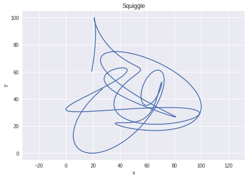
All the squiggles look like this:

The time variable is in the first column, with dt of 1/60 seconds, equal for all squiggles. Next columns are in pairs, x and y, with beta calculated for A=kC^beta, so that at beta=1, the speed is constant. The equations are not taken from Viviani and Stucchi paper, Alex and I derived them, but I assume they should be pretty similar, since they give correct results. The geometry or the shape of each squiggle is exactly the same, and the speeds of the dot are different. In regression analysis, with just logC as predictor and logA as criterion, the coefficient is very nearly the one set in the retrack function as “target beta”. That is, regression analysis, without taking D into account, returns precisely the beta that was used to generate the trajectory.

When adding log D to the regression analysis as a predictor, the coefficient for log C is 0.67, and for logD is 0.15, for all trajectories. I would interpret this result as a statistical artifact - the same one as in my post above, with random a and b)

RM: The power law has nothing to do with why the Viviani/Stucchi study makes sense from a control theory perspective and other power law studies don’t. The Viviani/Stucchi study actually tests for a controlled variable; other power law studies don’t. The fact that the hypothesized controlled variable in the Viviani/Stucchi study is a power coefficient is beside the point. At least it is treated as a hypothesis about a variable aspect of the movement that might be controlled. Power law studies just look at features of the movement itself under the assumption that this will tell them something about how the movement is produced; it won’t

First bold - agreed, the power law itself does not have much to do with controlled variables, but the valuable aspect of this study, and most other power law studies, is finding relatively strong laws in behavior. A correlation of 0.9 is not commonly seen in life sciences (“respectable, if not outstanding”). There is another study by Viviani testing position and velocity control model in 2d pursuit tracking. Viviani et al(1987): Following Powers (1978), one could, in fact, argue that the subject’s primary goal is not to produce a specified overt behavior (i.e., a specific trajectory) but rather to minimize the discrepancy between the actual and ideal value of the position error
link to pdf

I think there is another paper, but with ellipses and the same model. So, for the second bold, it is not true that people assume that the power law itself tells them something about how the behavior is produced. The power law is a descriptive model of behavior with a relatively narrow range, only fast movements; although sometimes the generality is a overstated. Still, it is perfectly clear that it is a description of behavior with an unknown explanation. People make all kinds of models that are supposed to be generating movements that fit some power law.

RM: It just struck me as a pretty amazing coincidence that in the equations above the power exponents of R and C --1/3 and 2/3, respectively – are exactly the exponents that have been proposed as those that characterize the power “law”; a law that, I believe, is presumed to reflect properties of nature (behavior), not of mathematics.

It is a pretty strange coincidence! It doesn’t look so amazing when you see that people can move at low speeds with absolutely no power law, or that for shapes that are not ellipses, when traced in fast and smooth manner, the exponent is reliably a very different value from the value found in ellipses and squiggles. It does not have to be 1/3 or 2/3. The exponent does reflect something about the behaving system, some kind of a limitation in control and production of speed, coupled with environment properties. This was determined by, again, Viviani, with drawing ellipses in water vs in air; or in children drawing vs adults drawing.

RM: Yes, unless all of the variance in the criterion variable (V or A) is accounted for by the included predictor (R or C). This would be the case, for example, in a perfect ellipse, which follows the power “law” exactly.

Not quite right - you can check with the squiggles - regression of logA and logC should give very nearly the exponent in the column name, and the r2 is near 1 for all of them, so there is no room or need for improvement. Same thing with ellipses.

[amatic]

AM: When adding log D to the regression analysis as a predictor, the coefficient for log C is 0.67, and for logD is 0.15, for all trajectories.

On second try, double checking, the coefficient for log (D) is 0.33 (using log base 10 in all cases), as it should be according to log(A) = 0.67 * log( C ) + 0.33 * log(D), or A = C^2/3 D ^1/3

AM: Should the omitted variable bias improve the prediction of the criterion variables from the predictors and the regression parameters?

RM: Yes, unless all of the variance in the criterion variable (V or A) is accounted for by the included predictor (R or C). This would be the case, for example, in a perfect ellipse, which follows the power “law” exactly.

Maybe not the squiggles because they have a near perfect power law law fit. What would be a good test case for this? Empirical data with not so great r² ? Are you saying that the prediction of A from C from the power law fit should be improved when using a different beta (calculated from multiple regression)?

Or that the prediction of A should be improved when using the coefficients from multiple regression from C and D? If yes, then why even do the multiple regression, both coefficients are known from the formula?

[rsmarken]

Hi Adam

RM: Or better yet could you just send me several columns of x,y coordinates of a spot moving in a squiggle pattern according to a power law with several different beta values?

AM: Here is an excel file with the squiggles: power_law_squiggles.xlsx

RM: Thanks Adam. As I said in private, I set up a spreadsheet analysis of that data and, sure enough, the single variable regression picks up all the beta values exactly. But there are some other features of the results that keep me suspicious if the use of regression as a way of analyzing curved movement trajectories.

1. While the single predictor regression picks up all beta values exactly, only the regression on the squiggle produced by a beta of .67 results in a prediction with constant D and no covariance between D and C.

2. The single predictor regression fails for all negative values of beta.

3. I am able to produce random squiggles (from low pass waveforms in X and Y) that result in beta values that are close to or exactly .67 but, unlike the results with the squiggle made with a beta of .67, the variance of D is pretty high as is the covariance between C and D. And the R^2 for these randomly produced squiggles with beta = .67 are around .9, unlike the R^2 for the single predictor regression for the squiggles produced with a beta of .67, which is 1.0.

RM: So there is still some mystery here. You have convinced me that, if a squiggle movement is produced with a single positive beta value, it would be picked up by the regression and you would know that because the single predictor R^2 would be 1.0.[ Now I realize it would just be VERY close to 1.0 but not exactly 1.0; see below]

AM: There is another study by Viviani testing position and velocity control model in 2d pursuit tracking. Viviani et al(1987): Following Powers (1978), one could, in fact, argue that the subject’s primary goal is not to produce a specified overt behavior (i.e., a specific trajectory) but rather to minimize the discrepancy between the actual and ideal value of the position error
link to pdf

RM: Thanks for the reference. It’s difficult for me to follow what their version on Powers’ model is and how they evaluated it. Maybe you could give a simplified explanation. It’s great to find that someone knew of Powers’ work and tried to test the model.

AM: I think there is another paper, but with ellipses and the same model. So, for the second bold, it is not true that people assume that the power law itself tells them something about how the behavior is produced.

RM: Yes, that’s very interesting. If you get a chance it would be great to see what their model is.

AM: The exponent does reflect something about the behaving system, some kind of a limitation in control and production of speed, coupled with environment properties. This was determined by, again, Viviani, with drawing ellipses in water vs in air; or in children drawing vs adults drawing.

RM: I showed some time ago that this difference can be accounted for as a result of a change in the feedback connection between output and controlled variable. The water results in a lower gain, higher slowing connection between output and controlled variable than does air and this is reflected in the coefficient of the “power law” as determined by single predictor regression.

RM: Yes, unless all of the variance in the criterion variable (V or A) is accounted for by the included predictor (R or C). This would be the case, for example, in a perfect ellipse, which follows the power “law” exactly.

AM: Not quite right - you can check with the squiggles - regression of logA and logC should give very nearly the exponent in the column name, and the r2 is near 1 for all of them, so there is no room or need for improvement. Same thing with ellipses.

RM: To my surprise there IS room for improvement! For the regression on the squiggle with beta = .67 I thought the R^2 was 1.0 but when I increase the number of decimal places it turns out that it is only .999900 and the variance in D is not 0.0 but .000151 and the covariance between C and D is also not 0 but .000339. Apparently this was enough difference to allow improvement of the R^2 from .999900 to 1.00000 when D was included in the regression. And when you do include D in the regression, the value for beta (for C) goes from 0.6669657 to 0.6666667, which is exactly 2/3, and the value for the coefficient of D is exactly 1/3.

RM: So the regression that includes both C and D as predictors of A actually does improve the prediction (in terms of R^2 and in terms of the actual values of the coefficients of C and D (curvature and affine velocity) that predict A (the speed of movement as angular velocity). This is true of all the squiggles made by the different betas (including the one’s made with negative beta). Including D always resulted in an R^2 of 1.000000 and coefficients for C and D of 2/3 and 1/3, respectively, as per the mathematics: log(A) = 2/3 * log( C) + 1/3 * (log(D).

RM: What this means to me is that it is impossible to make a curved trajectory with speed proportional to curvature (A = beta*C) without producing some variation in affine velocity (D). The degree of variation that results depends on the distance of beta from the true mathematical beta, 2/3; the closer beta is to 2/3, the smaller the variance in D. Indeed, when beta = .67 the variance in D is vanishingly small. But it’s there.

RM: I don’t know what all this means. I think it means that the results of a regression analysis relating C to A (or V to R) are problematic as descriptions of what a person is doing when they make curved movements.

RM: But what I would really like to see is a nice, clear description of Viviani’s Powers-inspired control model of tracking a squiggle movement and how it was evaluated.

Best

Rick

[amatic]

RM: But there are some other features of the results that keep me suspicious if the use of regression as a way of analyzing curved movement trajectories.

There are definitely issues with using regression to find power laws, many people mention the issues - using log functions is the first issue, as they increase the goodness of fit, there are issues with noise, there is some overgeneralization, etc.

RM: While the single predictor regression picks up all beta values exactly, only the regression on the squiggle produced by a beta of .67 results in a prediction with constant D and no covariance between D and C.

What is the issue? Did you expect constant D for all trajectories? Not sure I understand. There is no covariance because D is constant. In other cases D is not constant because both velocity and acceleration vectors that determine D are varying.

RM The single predictor regression fails for all negative values of beta.

Looks like this was a problem with the construction of trajectories, not with regression. I’ve used dt of 1/60 s before, now with 0.005s it works much better, even for negative betas: squiggles.xlsx

RM: I am able to produce random squiggles (from low pass waveforms in X and Y) that result in beta values that are close to or exactly .67 but, unlike the results with the squiggle made with a beta of .67, the variance of D is pretty high as is the covariance between C and D. And the R^2 for these randomly produced squiggles with beta = .67 are around .9, unlike the R^2 for the single predictor regression for the squiggles produced with a beta of .67, which is 1.0.

From random x and y, summed sinewaves I get different betas and r2. For example the the ‘original’ squiggle from the excel file had a beta of 0.74 and r2 of 0.9 between A and C. For V and R, the r2 is much lower. There are some issues with using A and C regression vs V and R regression (or V and C). I trust the V and R more.
The second issues, I guess, is that there might be influence of “noise”. That is - in some cases, the regression will give a speed-curvature power law where it does not exist.

RM: Thanks for the reference. It’s difficult for me to follow what their version on Powers’ model is and how they evaluated it. Maybe you could give a simplified explanation. It’s great to find that someone knew of Powers’ work and tried to test the model.
on page 71, they give the formulas:

Xp’’ is the acceleration in the x direction, alpha is the position gain, Xt is the target position (delayed), Xp cursor position. X’t is target speed and X’p cursor speed, beta is the velocity gain.
Same with Y.

This needs to be integrated to advance the program step, so after calculating x acceleration, calculate x velocity and x position, like this:
Xp’ = Xp’’ * dt
Xp = Xp’ * dt

The formulas are pretty similar to the standard proportional with slowing model. They say the velocity control is important, but it is more about position control (from what I remember when analyzing their model).

RM: I showed some time ago that this difference can be accounted for as a result of a change in the feedback connection between output and controlled variable. The water results in a lower gain, higher slowing connection between output and controlled variable than does air and this is reflected in the coefficient of the “power law” as determined by single predictor regression.

That is an interesting possibility, but first someone needs to find a controlled variable for drawing ellipses fast, because position control does not work in that case.

RM: So the regression that includes both C and D as predictors of A actually does improve the prediction (in terms of R^2 and in terms of the actual values of the coefficients of C and D (curvature and affine velocity) that predict A (the speed of movement as angular velocity). This is true of all the squiggles made by the different betas (including the one’s made with negative beta). Including D always resulted in an R^2 of 1.000000 and coefficients for C and D of 2/3 and 1/3, respectively, as per the mathematics: log(A) = 2/3 * log( C) + 1/3 * (log(D).

Well, try making two completely random variables A and C, no need to smooth them even. Then calculate a new variable D as D = A³ / C². Then do single predictor regression between log A and log C, it should give you no correlation, which is the correct result. Try multiple regression with log C and log D as predictors and log A as criterion, and it will give you 2/3 and 1/3 as coefficients and r2 = 1.0 - for any two random list A and C.

That can’t be interpreted as improving the prediction between A and C, they are both random.

RM: But what I would really like to see is a nice, clear description of Viviani’s Powers-inspired control model of tracking a squiggle movement and how it was evaluated.

Yeah, this might be a good idea for a journal club thread here on the forum, along with the second experiment where they did ellipse tracking.

[rsmarken]

Hi Adam

RM: While the single predictor regression picks up all beta values exactly, only the regression on the squiggle produced by a beta of .67 results in a prediction with constant D and no covariance between D and C.

AM: What is the issue? Did you expect constant D for all trajectories? Not sure I understand. There is no covariance because D is constant. In other cases D is not constant because both velocity and acceleration vectors that determine D are varying.

RM: Actually, it turns out that D is never constant for any value of beta. Although the variance of D decreases as you get closer to beta = .67 it never gets to 0. I wonder what would happen if you used beta equal to exactly 2/3 – the mathematical coefficient of
curvature, 0.666666666666667 according to my computer. The “problem” is just that, for curves generated by all values of beta so far, I find that when you include D as a variable in the analysis you always get the exact coefficients of in the mathematical formula, 2/3 for C and 1/3 for D.

RM: Still, the single predictor regression does pick up the beta that generated it. Maybe I could get a better handle on my problem if you could generate trajectories with different values of the coefficient for D rather than C. Could you do that?

RM: The single predictor regression fails for all negative values of beta.

AM: I’ve used dt of 1/60 s before, now with 0.005s it works much better, even for negative betas: squiggles.xlsx

RM: Yes, it does, thanks.

RM: Thanks for the reference. It’s difficult for me to follow what their version on Powers’ model is and how they evaluated it. Maybe you could give a simplified explanation.

AM: on page 71, they give the formulas:

AM: The formulas are pretty similar to the standard proportional with slowing model. They say the velocity control is important, but it is more about position control (from what I remember when analyzing their model).

RM: From a PCT perspective this is a very confusing (or confused) model. One controlled variable is the difference between target and cursor position, with an implicit fixed reference of 0, and the other is the difference between target and cursor velocity, also with an implicit reference of 0. These four error signals (two for the X and two for the Y dimension) are combined to produce an output that accelerates the cursor. This acceleration affects both the position and velocity of the cursor, so it affects both controlled variables, differentially affecting the size of the error in both variables.I don’t see how a single output (acceleration) can control both position and velocity at the same time. But perhaps there is such a high correlations between position and velocity that it works out.

RM: In PCT, each controlled variable would be handled by a separated control system. So the PCT equivalent of this model would require 4 control systems; 2 for control of cursor/target position and velocity difference in the X dimension and 2 for control of cursor/target position and velocity in the Y dimension.

RM: It would probably make sense to arrange these control systems hierarchically so that the position control systems are above the velocity control systems so that the outputs of the position controllers would set the reference for the velocity controllers and the outputs of the velocity controllers be the acceleration variable that affects the cursor.

RM: One nice thing about the PCT approach, besides the fact that it would probably fit the Viviani data perfectly, is that it makes clear what variables are being controlled. Also, it allows for the possibility that the subject may vary their reference for the state of the highest level variable (since the reference variables are assumed to be 0 and constant they are not even shown in the Viviani equations – a rather significant omission in a model that is presumably inspired by Powers’ work. So you could ask the subject to control for the cursor being, say, 1 cm to the left of the cursor, and the model can easily account for the fact that that happens.

AM: … try making two completely random variables A and C, no need to smooth them even. Then calculate a new variable D as D = A³ / C². Then do single predictor regression between log A and log C, it should give you no correlation, which is the correct result. Try multiple regression with log C and log D as predictors and log A as criterion, and it will give you 2/3 and 1/3 as coefficients and r2 = 1.0 - for any two random list A and C.

AM: That can’t be interpreted as improving the prediction between A and C, they are both random.

RM: No it can’t. It is simply improving your prediction of A and giving you the correct coefficients for the equation that relates C and D to A.

RM: But what I would really like to see is a nice, clear description of Viviani’s Powers-inspired control model of tracking a squiggle movement and how it was evaluated.

AM: Yeah, this might be a good idea for a journal club thread here on the forum, along with the second experiment where they did ellipse tracking.

RM: Actually, you already gave a nice description of it in the two equations above. But it would be nice to have a discussion of the difference between Viviani’s Powers-inspired control model and what a Powers control model might actually look like.

RM: But let me know if you can generate some trajectories from D (affine velocity) with different coefficient values.

Best

Rick

[amatic]

AM: That can’t be interpreted as improving the prediction between A and C, they are both random
RM: No it can’t. It is simply improving your prediction of A and giving you the correct coefficients for the equation that relates C and D to A.

Why even do the regression analysis if you already have C and D and their coefficients? You can just calculate A.

RM The “problem” is just that, for curves generated by all values of beta so far, I find that when you include D as a variable in the analysis you always get the exact coefficients of in the mathematical formula, 2/3 for C and 1/3 for D.

Yep. That is the problem. Multiple regression works also for random values of A and C, any beta, any r2, and any coefficients, In other words, not only for curves, but for all situations where D is defined as D = A³ / C², the coefficients of log D and log C will be 2/3 and 1/3.

RM: Still, the single predictor regression does pick up the beta that generated it. Maybe I could get a better handle on my problem if you could generate trajectories with different values of the coefficient for D rather than C.

Try random variables. It works perfectly. Define a and b as lists of random numbers, should be possible in excel. Then define a third variable c as c = a^m / bⁿ . When you solve for a, you will get
a^m = c * bⁿ, then
a = c^1/m * b^n/m
log a = (1/m) log c + (n/m) log b

For any random variables a and b, and for and coefficients m and n, multiple regression with log c and log b as predictors will always return perfect fit with coefficients 1/m and n/m.

RM: Actually, it turns out that D is never constant for any value of beta. Although the variance of D decreases as you get closer to beta = .67 it never gets to 0. I wonder what would happen if you used beta equal to exactly 2/3

In an ellipse made from sine waves, you can get a constant or near constant D.

RM: From a PCT perspective this is a very confusing (or confused) model. One controlled variable is the difference between target and cursor position, with an implicit fixed reference of 0, and the other is the difference between target and cursor velocity, also with an implicit reference of 0. These four error signals (two for the X and two for the Y dimension) are combined to produce an output that accelerates the cursor. This acceleration affects both the position and velocity of the cursor, so it affects both controlled variables, differentially affecting the size of the error in both variables. I don’t see how a single output (acceleration) can control both position and velocity at the same time.

Integrate the acceleration and you get velocity. Then you integrate velocity and get position.

RM: In PCT, each controlled variable would be handled by a separated control system. So the PCT equivalent of this model would require 4 control systems; 2 for control of cursor/target position and velocity difference in the X dimension and 2 for control of cursor/target position and velocity in the Y dimension.

They are conceptually separated, but in the formulas they come down to the same thing, if you play a bit with the algebra. There are still 4 controlled variables.

[rsmarken]

Hi Adam:

AM: Why even do the regression analysis if you already have C and D and their coefficients? You can just calculate A.

RM: That’s what I was thinking. But I think you have demonstrated that the single predictor regression of curvature on speed can pick up something close to the beta value for the relationship between these variables. In other words, you have convinced me that I was wrong to say that the power law is a statistical artifact. I think it’s clearly a side effect of control but it’s not a statistical artifact. I think the best explanation of the “power law”, such as it is, was given by Richard Kennaway, who showed that it is a relationship between speed and curvature that is an expected side-effect of any smooth periodic function, as shown here:

RM: This means that the “power law” will characterize curved human movement to the extent that people tend to move their limbs in smooth, periodic trajectories, like those shown above. Why do people move this way? I think the answer may lie in the results of the Viviani/Stucchi experiment in which constant velocity motion was perceived when the motion was generated by something close to a 2/3 “power law”. That is, constant velocity motion was perceived when the measured velocity of motion was slower for steep than for shallow curves. This suggests that one variable being controlled when a person is controlling for producing a constant velocity motion is the relationship between speed and curvature. For example, one possible controlled variable could be a function of the product A * C. In order to keep this product (the perception of motion) constant A and C must vary inversely in a power relationship. At least it’s a starting hypothesis about one of the variables people might control when hey move their limbs in curved trajectories.

RM: Re The Viviani/Campadelli model I said: In PCT, each controlled variable would be handled by a separated control system. So the PCT equivalent of this model would require 4 control systems; 2 for control of cursor/target position and velocity difference in the X dimension and 2 for control of cursor/target position and velocity in the Y dimension.

AM: They are conceptually separated, but in the formulas they come down to the same thing, if you play a bit with the algebra. There are still 4 controlled variables.

RM: I suppose that’s possible, though it’s not clear to me how 4 input variables can all be controlled simultaneously with only 2 output degrees of freedom. But even if that is possible, the model, as written,

hides what I think is a very important difference between PCT and other applications of control theory to behavior: the “secularly” (autonomously) adjustable reference specifications for the state of the controlled variables. These reference variables would appear after the formulas for the controlled variable. For example, one controlled variable in the above equations is X.T - X.P – the distance from target (T) to cursor ( P) in the X dimension. In the equation above, the PCT version of the formula for the X output based on X.T - X.P would be alpha*((X.T - X.P) - 0), where 0 is the assumed fixed value of the reference specification for (X.T - X.P). The more general way to write it would be alpha*((X.T - X.P) - R) where R is the reference variable that can be autonomously adjusted to any constant or variable value by the person doing the tracking. It might be nice to repeat the Viviani/ Campadelli tracking experiment with the subjects asked to keep the cursor some distance to the left, right , above or beneath the target.

RM: I hope I’ve given you some ideas about directions you might go in developing a PCT based control theory approach to understanding the control of movement.

Best

Rick

[amatic]

RM: But I think you have demonstrated that the single predictor regression of curvature on speed can pick up something close to the beta value for the relationship between these variables. In other words, you have convinced me that I was wrong to say that the power law is a statistical artifact. I think it’s clearly a side effect of control but it’s not a statistical artifact.

Great.

RM: I suppose that’s possible, though it’s not clear to me how 4 input variables can all be controlled simultaneously with only 2 output degrees of freedom.

You can always try the model and see how it works. Some pointers you can find in Bill’s NonAdaptive demo, which also has speed and position as controlled variables but force as output. Although, the speed is not the rate of change of cursor-target distance, but the rate of change of cursor position. Also, there are absolutely no rules against putting the formulas in a single line, if you prefer. The computer does not mind. The same goes for the reference signals - if they are assumed to be zero, you don’t write them, perfectly fine.

This is Bill’s code and comments from that demo:
procedure TMainForm.RunModel;
begin
// acceleration = applied force minus velocity and spring feedback, over mass
Accel := (Force + ForceDist - D * Vel - S * Pos)/M;
LastPos := Pos; // save position for computing velocity
// New position = old position + velocity * dt + 1/2 acceleration * dt-squared
Pos := Pos + (Vel + 0.5 * Accel * dt) * dt;
Vel := Vel + Acceldt; // update velocity; dt is time step per iteration
VelFB := (Pos - LastPos)/dt; // compute velocity from delta-pos
e3 := SepRef - (Pos - Target); // pos - target is actual separation
e2 := PosGain * e3 - velfb; // posgaine3 is output of position control system
Force := VelGain * e2; // which is the velocity reference signal
end;

The control systems output the last line, so working backward:
Force = VelGain * e2. /// replace e2
Force = VelGain * (PosGain * e3 - VelFB) // replace e3 and VelFB
Force = VelGain * (PosGain * (SepRef - (Pos - Target)) - (Pos - LastPos)/dt)
Force = VelGain * PosGain * (SepRef - (Pos-Target)) - VelGain* (Pos-LastPos)/dt // now assume sepref = 0
Force = VelGain * PosGain * pos_error - VelGain * vel

So, the system is not identical, but it is not that different. Both are second-order systems (highest derivative being the acceleration, the second derivative of position) analogous to the mass-spring-damper system.

As for them forgetting the reference signal, they don’t, they just assume it is zero. here is a quote:

Thus, within the general framework proposed by Powers for describing purposive systems, we would identify the system input with the position error vector delta S, the system output with the pursuit position; the target position takes the role of an external disturbance that moves the input away from its ideal internal reference (delta S = 0, under the stated assignments).

[rsmarken]

Hi Adam

RM: I suppose that’s possible, though it’s not clear to me how 4 input variables can all be controlled simultaneously with only 2 output degrees of freedom.

AM: You can always try the model and see how it works. Some pointers you can find in Bill’s NonAdaptive demo, which also has speed and position as controlled variables but force as output. Although, the speed is not the rate of change of cursor-target distance, but the rate of change of cursor position. Also, there are absolutely no rules against putting the formulas in a single line, if you prefer. The computer does not mind. The same goes for the reference signals - if they are assumed to be zero, you don’t write them, perfectly fine.

AM: This is Bill’s code and comments from that demo:
procedure TMainForm.RunModel;
begin
// acceleration = applied force minus velocity and spring feedback, over mass
Accel := (Force + ForceDist - D * Vel - S * Pos)/M;
LastPos := Pos; // save position for computing velocity
// New position = old position + velocity * dt + 1/2 acceleration * dt-squared
Pos := Pos + (Vel + 0.5 * Accel * dt) * dt;
Vel := Vel + Acceldt; // update velocity; dt is time step per iteration
VelFB := (Pos - LastPos)/dt; // compute velocity from delta-pos
e3 := SepRef - (Pos - Target); // pos - target is actual separation
e2 := PosGain * e3 - velfb; // posgaine3 is output of position control system
Force := VelGain * e2; // which is the velocity reference signal
end;

AM: The control systems output the last line, so working backward:
Force = VelGain * e2. /// replace e2
Force = VelGain * (PosGain * e3 - VelFB) // replace e3 and VelFB
Force = VelGain * (PosGain * (SepRef - (Pos - Target)) - (Pos - LastPos)/dt)
Force = VelGain * PosGain * (SepRef - (Pos-Target)) - VelGain* (Pos-LastPos)/dt // now assume sepref = 0
Force = VelGain * PosGain * pos_error - VelGain * vel

AM: So, the system is not identical, but it is not that different. Both are second-order systems (highest derivative being the acceleration, the second derivative of position) analogous to the mass-spring-damper system.

RM: This will take days for me to try to decipher (I am not the sharpest crayon in the box, after all). I think it would help me out (as well as any other similarly sharpness - challenged onlookers) if you could show me the functional diagrams of the two systems so that I can compare them. But as best as I can tell at first glance, it seems like in Bill’s system the reference for the velocity control system – posgain*e3 – is a variable, computed as the output of the position control system, whereas the reference for velocity control in the Viviani/Campadelli model is a constant, 0. If the reference for the velocity control system in your program implementation of the Viviani and Campadelli model is a variable (it’s hard for me to tell) then I don’t think your program is equivalent to the Viviani/Campadelli model. But I have been known to be wrong before;-)

AM: As for them forgetting the reference signal, they don’t, they just assume it is zero. here is a quote:

V/C: Thus, within the general framework proposed by Powers for describing purposive systems, we would identify the system input with the position error vector delta S, the system output with the pursuit position; the target position takes the role of an external disturbance that moves the input away from its ideal internal reference (delta S = 0, under the stated assignments).

RM: This is very interesting. They do seem to understand that Powers model has an autonomously set reference specification for input, though their equations imply that both position and velocity are inputs with references fixed at 0. Why don’t they mention the velocity control system?

RM: Other than that this Viviani and Campadelli model looks like a perfectly fine perceptual control model. I’m sure it could produce movements that result in something close to a power law relationship between curvature and velocity. Is there something wrong with this model? I produced essentially this model as the PCT explanation of the power law (as a side effect of control) when Alex asked how PCT would explain the power law and he hit the ceiling. The only difference between my model and that of Viviani and Campadelli (other than that mine did compensatory rather than pursuit tracking) is that it controls position relative to a varying reference. I guess Alex thought that the varying reference was “cheating” in some way but I think it was on the right track, as is Viviani/Campadelli model.

Best

Rick

[amatic]

RM: This will take days for me to try to decipher (I am not the sharpest crayon in the box, after all). I think it would help me out (as well as any other similarly sharpness - challenged onlookers) if you could show me the functional diagrams of the two systems so that I can compare them. But as best as I can tell at first glance, it seems like in Bill’s system the reference for the velocity control system – posgain*e3 – is a variable, computed as the output of the position control system, whereas the reference for velocity control in the Viviani/Campadelli model is a constant, 0. If the reference for the velocity control system in your program implementation of the Viviani and Campadelli model is a variable (it’s hard for me to tell) then I don’t think your program is equivalent to the Viviani/Campadelli model. But I have been known to be wrong before;-)

References for velocity in both models are set by the output of the position model. What I’ve tried to show is how to make Bill’s code for the control systems fold into one line by replacing named variables with expressions they equal. You can write a system of formulas in two lines:
a = b + c
d = a + q

or you can write them in one line, with the variable you care about or ‘solve for’ one the left side.
d = b + c + q

That is all I did with Bill’s code, and it comes to a form similar to Viviani’s. The difference between the models is the calculation of velocity (I’ve mentioned).

RM: Is there something wrong with this model?

It works only for squiggles, and following squiggles does not result in consistent power law exponents or r2s. There are some other issues with the implementation, but I would need to double-check that.

RM The only difference between my model and that of Viviani and Campadelli (other than that mine did compensatory rather than pursuit tracking) is that it controls position relative to a varying reference. I guess Alex thought that the varying reference was “cheating” in some way but I think it was on the right track, as is Viviani/Campadelli model.

I can think of several objections for the varying reference proposal.

(1) A reference is an output of a higher-level control system. If it is not specified how and why the reference forms, that is not a solution but simply transferring the problem to a different place. The problem is still what are the controlled variables at this level that creates a varying reference for the position or distance control level.

(2) It does not work. For the speeds where the power law appears consistently, the position control system does not follow the reference - it creates much bigger shapes than the reference shape, just like tracking fast targets. A quick and dirty solution is to have a smaller reference ellipse, and this works somewhat, but there is again the problem of matching subject speed or rhythm. This can be solved, but still, the solution does not work for shapes other than ellipses.