[Bruce Nevin 2018-07-19_09:46:11 ET]
Martin Taylor 2018.07.17.17.16 –
Rick, Martin listed “eight … falsehoods you incorporated in your rebuttal.” You replied “they are not “falsehoods” but the best we could do to understand your criticisms.” That seems to affirm that you did not understand his criticisms very well.Â
I know of two ways to demonstrate understanding, and both of them involve a test of understanding that is akin to the Test for controlled variables. One of the two ways is to apply what is understood. This demonstrates control of the perceptions intended by the words. The other way is to paraphrase in different words and ask if the paraphrase is correct. This is similar to e.g. the Coin Game.
Would it be a fair paraphrase of your to enclose each of the eight pairs (statements in Martin’s list and your rejoinders to them) in this frame?
When you said [quote from Martin’s rebuttal] it appeared to us that you meant [quote from your rebuttal of the rebuttal]. Is that what you intended? If so, [further rebuttal].
You actually did this, in effect, at this point of your reply:
It seems to me, naively, that this is not an accurate paraphrase. I think Martin’s point isÂ
a. that one form of the equation is a generalization across all possible velocities,Â
b. that the other form of the equation can be applied only to particular velocity data from a particular experiment, andÂ
c. that you employed the latter (b) as though it were equivalently (a) a generalization across all possible velocities.
Only Martin can say whether or not I have accurately paraphrased what he wrote. If he affirms that I did, are these paraphrase statements incorrect?
I think you have a kind of important typographical error here:
I think you meant to say “we said that your critique was based on your misunderstanding of those equations.” Is that correct? Are there possibly other misstatements confusing the discussion?
···
Rick Marken 2018-07-17_10:31:31 --​
This dispute seems at last to be converging toward common perceptions of what is in dispute, but I still am not understanding it.
RM: What you are saying is that we made the mistake of taking the dot derivatives in the two Gribble/Ostry equations as being time derivatives.
RM: No,
​​
we said that your critique was based on our misunderstanding of those equations. Specifically that the derivatives in the curvature equation were different from those in the velocity equation. Your claim that these derivatives are different is simply wrong and, thus, invalidates your mathematical critique from the get go.
[Rick Marken 2018-07-17_10:31:31]
[Martin Taylor 2018.07.16.15.12]
MT: As well you have known for a very long time, I haveinsufficient hubris to attempt a model of observed
behaviour before trying the TCV to figure out what
variable(s) might be being controlled during the task. I
have no means to do the TCV needed, so I refrain from
suggesting a model. You are not so inhibited.
RM: You have to have had some idea of what the
controlled variable might be when people make curved
movements or you wouldn’t know that the power law is
"almost certainly a side-effect in any
of the experiments that find velocity to have a near
power-law relationship to the radius of curvature ",
as you note in your rebuttal. In PCT, a “side-effect” is a
relationship between variables that exists because a
variable is under control but this relationship not part
of the process that results in control of that variable.
For example, the relationship between disturbance and
output in a tracking task is a side effect of controlling
the position of the cursor but is not part of the process
that results in control of cursor position. In order to
know that the power law is, indeed, a side-effect, you had
to have an idea of what variable is under control when
people make curved movements as well as having an idea of
how the instantaneous curvature and velocity of these
movements are related to this variable. This should have
been enough to let you develop a first approximation to a
model of curved movements that would demonstrate why the instantaneous
curvature and velocity of these movements is a side
effect of controlling this variable. The model itself
would have been a basis for the TCV; it would be a test
of the correctness of your hypothesis regarding the
variable under control. So it would not have been
hubris to model the behavior before doing the TCV since
you presumably had to have had the essential components of
the model in mind when you said that the power law is
almost certainly a side effect.Â
MT: For the record, here are justeight of the falsehoods you incorporated in your
rebuttal of my comment on the Marken and Shaffer paper
(copied from [Martin Taylor 2018.03.08.23.07]). Despite
having been made aware of their falsity, yet you
continue to repeat some of them on CSGnet. Why do you do
that?
RM: Because they are not "falsehoods" but the best we
could do to understand your criticisms.
Â
----------begin quote (replacingreferences to “you” with references to “they”, and added
numbering)-------* MT: (1) In the very first paragraph you claim that myreason for writing a critique was that the idea that
the power law might be a behavioural illusion caused
“consternation”, whereas I made explicit that nothing
in my critique had any bearing on that issue. Indeed,
I finished my critique with the statement that perhaps
the power law is indeed a behavioural illusion, though
M&S sheds no light on that issue.*
RM: Since, as I noted above, you came up with no
hypothesis about what variable might be controlled, I
dismissed your claims of accepting that the power law is a
behavioral illusion because you gave no evidence of
understanding what a behavioral illusion is.
Â
MT: (2) M&S say that mycritique of their use of Gribble and Ostry’s equations
is based on my belief that those equations are wrong
or misleading, whereas I pointed out that they are
well known and universally accepted equations for
using observed data to measure the velocity (equation
- and curvature (equation 2) profiles observed in an
experiment. Neither Gribble and Ostry nor (so far as I
know) anyone other than Marken and Shaffer ever
claimed that the observed velocity was the only
velocity that could be used to get the correct
curvature from the equation for R.*
RM: No, we said that your critique was based on our
misunderstanding of those equations. Specifically that the
derivatives in the curvature equation were different from
those in the velocity equation. Your claim that these
derivatives are different is simply wrong and, thus,
invalidates your mathematical critique from the get go.
Â
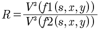
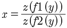
MT: (3) I never said that thederivation of V = R**1/3D1/3** was wrong. I said that since the formula for D was
velocity (V) times a constant in spatial variables,
the equation is not an equation from which one can
determine V. The M&S claim that it is an equation
from which one can determine V is the core of my
critique.*
RM: And we never said that you said that the derivation
of
-
V
= R**1/3D1/3**Â * was
wrong. We said that what you said about it not being an
equation that can be used to predict V using linear
regression is wrong. Which it is.Â
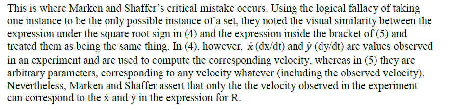
MT: (4) M&S falsely claim that I argue that“it should have been obvious that X-dot and Y-dot are
derivatives with respect to time in the expression for
V, whereas they are derivatives with respect to space
in the expression for R (p. 5)”. On the contrary, I
devote the first couple of pages of my critique to
showing why, despite the radius of curvature being a
spatial property, nevertheless it is quite proper to
use time derivatives in the formula for R.*
RM: But that’s what you argued, right here:Â
RM: What you are saying is that we made the mistake of
taking the dot derivatives in the two Gribble/Ostry
equations as being time derivatives. But that was not
mistake. The mistake is all yours.
MT: (5) M&S say that becauseGribble and Ostry correctly transformed Viviani and
Stucchi’s expression for R using spatial derivatives
into one using time derivatives (a derivation with
which I started my comment), therefore they were
correct to say that ONLY the velocity found in an
experiment can be substituted into the numerator of
the expression for R, whereas both my derivation and
that of Viviani and Stucchi (essentially the same)
makes it crystal clear that this is not true.*
RM: Well, that would be news to all the power law
researchers who computed velocity and curvature the way I
did in my analyses, using time derivatives.
Â
MT: (6) M&S follow thisastounding assertion with an couple of paragraphs to
show why the V = R**1/3D1/3** equation is correct, implying that my comment claimed
it to be wrong. Early in my comment, however, I wrote:
“They then write their key Eq (6) [V = R**1/3D1/3** ],
which is true for any value of V whatever…” Any
implication that my comment claimed the equation to be
incorrect is false.*
RM: What we showed is that that equation has been used
by others to show what we showed in our paper – that
using only R (curvature) as the predictor in a regression
on V (speed) – will result in an estimate of the power
coefficient of R that deviates from 1/3 by an amount
proportional to the correlation between R and D (radial
velocity).Â
Â
MT: (7) Omitted Variable Bias:My comment demonstrated that the finding predicted and
reported by M&S was actually a tautology having no
relation to experimental findings, which will always
produce the result claimed by M&S to be an
experimental result. M&S in the paper and in the
rebuttal treat it as a discovery that can be made only
by careful statistical analysis, and do not
acknowledge the tautology criticism at all.*
RM: Your demonstration that our findings are a
“tautology” made no sense to us. You made this claim based
on your derivation of an equation for V of the form V = V.
But this is true for any equation. If X = f(Y) then you
can substitute X for the right side of the equation and
write the equation X = X. That’s not a tautology; that’s
just an irrelevant observation.
MT: (8) M&S: "At the heart of the criticismsof our paper by Z/M and Taylor is the assumption that
the power law is a result of a direct causal
connection between curvature and speed of movement or
between these variables and the physiological
mechanisms that produce them." I have no idea how this
astonishing statement can be derived from my
exposition of the mathematical and logical flaws in
their paper. My comment is designed to refute exactly
M&S’s claim of my motivation. The comment shows
that there is NO necessary relationship, causal
connection or otherwise, between curvature and speed
of movement.
*
RM: You were apparently trying to show, mathematically,
that the curvature and velocity of a curved movement are
physically independent, like the disturbance and output in
a tracking task. Since you didn’t speculate about the
controlled variable that might be simultaneously affected
by these two variables I assumed that you were dong this
to justify the assumptions of power law researchers that
these two variables are either causally related or
simultaneously caused by a third variable.Â
Â
--------end quote-------
MT: I repeat from my last message: *"* What's theadvantage to you of refusing to deal with scientific
points people bring up about your work?"
RM: We dealt with your confusing rebuttal as best we
could. There was nothing scientific about it inasmuch as
it was purely mathematical.
Best
Rick
Â
Well, I guess predictions aren't always wrong,and I am indeed not surprised.
Martin
–
Richard S. MarkenÂ
"Perfection
is achieved not when you have
nothing more to add, but when you
have
nothing left to take away.�
  Â
            Â
–Antoine de Saint-Exupery
Best
Rick
Â
What's theadvantage to you of refusing to deal
with scientific points people bring up
about your work? In what perception
you control would it create error if
you were to accept normal mathematics
or physics as being valid? When your
work is good, it’s good, but when you
make a mistake, why does it seem so
difficult for you to correct it? In
the curvature paper none of the
criticisms were relevant to a PCT
interpretation, but you make out that
all of them were intended to refute a
“correct PCT analysis” of the
experimental findings. Why?I don't expect an answer to a questionraised, but I wouldn’t be surprised at
an answer to something completely
different.