Thanks everyone, this discussion is adding nicely to the research paper. It’s priceless reading Bill’s 2005 ideas and I wish we’d had them already to quote in the article as he converged in a similar solution!
I do hope Rick has realised that the original paper already describes neatly everything he mentioned in detail - the TCV, the fact that it is a present time composite perception, the leaky integrator and the model fit with each individual participant. I think we all agree that adding an unseen disturbance and showing the PCT model advantage would have made a clearer point about the uniqueness and superiority of a PCT model. However, Rick has done plenty of that excellent research already!
All the best
Warren
Hi Adam,
Great work!
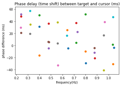
Yes, some participants exhibited phase advances and these tended to increase in likelihood as the cursor reached the sinusoid maximum (or minimum), that could be as a result of delayed sampling of velocity as during target deceleration, or as a result of overshoot - though in your track, as you said, the amplitude ratio seems about 1:1. Oher authors have also found shorter phase delays than I did (I found average 50ms for sines).
It looks like the tracking method you’re using is much more stable than the joystick we used. Probably not surprising given participants’ prior experience with these and fewer weird dynamic properties of the joystick that come in to play in our experiments. Later on we used a steering wheel for 1d tracking which was much smoother.
With respect to optimal parameters, it depends heavily on the transport delay you give the model and the phase delay the participant is exhibiting. In matlab I tend to use lsqnonlin to fit the parameters to a given trace. I think there is a sample script using this algorithm to estimate parameters of a position control model in Matlab on my GitHub page: Tracking_Matlab/test_opt_pos.m at master · maximilianparker/Tracking_Matlab · GitHub
In any case, I’m glad the model generalises well to your tablet task!
To add to the Bill quotes, Martin Taylor used a similar model in the modafinil and tracking conference paper ‘Effects of Modafinil and Amphetamine on tracking performance in sleep deprivation’, definitely worth a read!
Yes, I have looked at Simulink a little, definitely a good way to visualise the models. Bruce Abbott was experimenting with it a while ago too and also wrote both position and made a simulation of both position control and extrapolation models.
All the best,
Max
MP: With respect to optimal parameters, it depends heavily on the transport delay you give the model and the phase delay the participant is exhibiting.
I’ve tried fitting the extrapolation model to pseudorandom tracking. I also got no improvement or very slight improvement over the distance control only model (both findings replicated). It is strange. There is the information of target velocity available to the subjects, and they are not using it?
In the TrackAnalyze program, fitting a model is something like measuring the properties of the subject. So, if the model with 130ms of transport delay fitts best, we say that the subject probably has ~130ms of transport delay in the distance control loop. That is what we get for pseudorandom targets. For step-jumps or square waves (if they are not periodic) we get larger estimates of transport delay using the distance control model. The target just appears up or down, there is no velocity information.
Maybe that is the “real” transport delay. Could it be that in procedures such as TrackAnalyze, we are underestimating the transport delay in pseudorandom tracking, because we are using a model that does not use velocity extrapolation, while the subjects are using it? Well, just guessing.
Excellent that both findings were replicated. Yes, exactly, it seems a strange proposition that the participants do not use velocity for pseudorandom targets. I had assumed that the utility of extrapolation should be negatively correlated with acceleration or deceleration. If the target velocity is changing quickly and often then delayed estimate of velocity should be inaccurate, and so the extrapolated position becomes less accurate. Based on this assumption, increasing target signal frequency (or frequencies for pseudorandom targets) should lead to reduced use of velocity extrapolation perhaps? However, your finding that phase delay decreases as frequency increases in sinusoids doesn’t really support that. I can’t imagine phase reduces for pseudorandom targets in that way though.
Yes, we also collected some unpredictable step wave data though I haven’t analysed it much yet it is clear that the time between target jump and the beginning of detectable movement are long. As you say, these are ‘pure’ in the sense that there can only be positional feedback. However, they do seem a little bit too long to be just the transport delay though, perhaps there is an additional time cost in driving movement from still (as well as inertia which obviously affects the delay across the movement).
I think it could be the case that we are underestimating transport delays, but there is some strong evidence in reaching studies that transport delays can be pretty fast, I think 80ms was the fastest estimate i’ve seen but usually in the region of 100-150ms.
Cheers,
Max
If the phase difference is in milliseconds and not in degrees (like in the previous plot), it remains near zero on average, maybe slight delay. Looking at just x wave forms of cursor and target:
Looks pretty random, but also short.
Another thing - did you ever have a trial with a sudden target jump during tracking a sinusoid? As in, tracking a sinusoid for half a minute in one place, then the target jumps to another place? Or disappears?
No, not really. Although I remember when I was speaking to Joost Dessing at that Measuring Behavior conference he thought it would be good look into it. We were talking about the idea that the overshoot in tracking is due to inertia in the limb rather than part of the control strategy per se. He was suggesting testing the idea with ‘jumps’ in target location during the sinusoid/pseudorandom. I can’t remember what exactly he expected to see in behaviour there though to test that assumption. Any idea? I think also he was suggesting a sort of impulse away from the sine and then back to it, rather than adding a step input signal to a sinusoid, if that makes sense?
A small note about the entire discussion so far. Two points:
(1) Bill’s own later simulations often had either velocity or acceleration as the lowest level of control.
(2) In off-line spreadsheet work with Bill P 10 or 20 years ago, I compared Bill’s own tracking data with band-limited “white noise” or “pink noise” disturbances (I don’t remember which or whether the tracking was was pursuit or compensatory, or how much transport lag we used or found) against the performance of an ideal tracker, using the autocorrelation function of the disturbance to generate the ideal using just position, position and velocity, and position, velocity, and acceleration. Bill’s actual performance exceeded the ideal tracker’s performance unless at least velocity was included. Including acceleration made the ideal tracker perform a little better. Both velocity and acceleration imply prediction.
These historical facts seem relevant, despite not having been published. I hope they help further discussion.
Hi Martin, nice to hear from you. I think that If we say that velocity and acceleration ‘imply prediction’ when used as controlled input variables, then we might as well hand the towel in! The way that most non-pct researchers use the term ‘prediction’ is not the same…
MParker: He was suggesting testing the idea with ‘jumps’ in target location during the sinusoid/pseudorandom. I can’t remember what exactly he expected to see in behaviour there though to test that assumption. Any idea? I think also he was suggesting a sort of impulse away from the sine and then back to it,
I don’t remember much, but the reactions to jumps might be different when the CV is at a lower level, and when it is at a higher level. Sometimes we might be controlling c-t distance, or c-t distance + t velocity; this would be the lower level. And other times, we might be controlling amplitude and frequency of movement by varying some oscillator and the output of the oscillator is a reference to the c-t distance system.
Assuming that the transport delay is longer in the higher-level loop than in the lower level loop, the phase shift between the disturbance input step (step in the target) and the output cursor step (step in the cursor) will be longer when controlling for amplitude and frequency, than when controlling for c-t distance + t velocity.
The problem is that phase shifts are already very long in step tracking, so if there is a long shift after a step during sine tracking, we wouldn’t know if it comes from controlling at a higher level, or from whatever process is causing the long phase shifts in regular step tracking, like inertia or some muscle nonlinearities or whatever.
That’s an interesting idea. Could you remind me a little of how you model the oscillator?
I have just tried to implement a similar thing, maybe different to what you mean here, but I thought that if the model uses memory of the previous positions of the target (memory) it can effectively fit a sinusoid to this ‘memory trace’ and then look up the target position on this trace (accounting for the transport delay), nulling the distance. I had imagined this to operate in parallel to position control which would be the default option. But is effectively two position controllers, one c-t and one c-t_hat where t_hat is the oscillator memory estimate of the current position of the target.
I imagine that the memory system would have to introduce some noise because in target occlusion studies the participants are not good at replicating the frequency of the sinusoid over the occlusion. However, it would presumably be less affected by noise in the input signal than the c-t controller.
Of course, even in the parallel control version they could have different transport delays…
Interesting. I wonder whether there is such a long phase shift following a step within a sinusoid target signal. If it was shorter than the ‘pure’ delay when tracking step signals maybe that would help us exclude possibilities for the long delay in step tracking.
Warren,
The way most non-pct researchers use the term “perception” is not the same either. Surely “prediction”, to everybody, implies using expectation about things that have not yet happened as part of the current set of perceptions that affect control. How far ahead those predictions go depends on the distribution of probable states x milliseconds, hours, years, or mega-years in the future. In simple tracking, the transport lag sets the minimum prediction time to be used, even in simple position control.
What limits the accuracy of prediction for, say, simple pursuit tracking, is the autocorrelation function of the disturbance, the variance accounted for by knowledge of the current value of a variable. The variance unaccounted for is the limit to prediction accuracy x time-units in the future, counting from the time of the most recent observation. Of course, the autocorrelation function itself cannot be determined without prior observations, just as the velocity and acceleration need prior observations for their determination.
In an experiment, however, the experimenter who designed the disturbance noise knows the autocorrelation function, so can be sure of the actual limits of prediction possible to an ideal tracker. It depends on the equivalent white noise bandwidth. For a sine-wave disturbance, for example, the equivalent bandwidth from the experimenter’s point of view is zero, and the ideal would be able to predict infinitely far into the future. With such a sine-save disturbance, any failure of a tracker in practice must include the inability of the perceiving apparatus to determine the equivalent disturbance bandwidth. The “failure to predict” noise of inability to use the experimenter-constrained bandwidth should be included along with other noise sources around the control loop when analyzing deviations from ideal tracking performance.
Now, perhaps we can extrapolate this to vastly different time scales, and recognize that it is in the everyday sense of “prediction” that astronomers tell us that in (If I remember correctly) 5 billion years, the Andromeda Galaxy will collide with our Milky Way. For the observations that lead to such a prediction, the disturbances are slow, with autocorrelation functions stretching billions of years into the future (so far as astronomers can determine).
Not all disturbances can be reduced to an equivalent white noise. For example, in most countries an election is a source of disturbance to the perceived structure of the Government. In some countries, such as the USA, it is almost certain there will be no federal election in the next few days after one was completed, or in the next few months, but in the few days around exactly two and exactly four years after one election, another is almost certain to occur. That disturbance is highly predictable in its timing, but its magnitude and direction is not. They are the only uncertainty in predicting how the structure of the Government may change. In other countries, the time of the next election is less precisely predictable (i.e. that an election will be held during a specified week is near zero for any week for a while after an election event, then rises until it become near unity by the legally limited life of the Government).
Maybe I have made the point. When the disturbance statistics are not rhythmic, velocity and acceleration are reasonable proxies for predictability, and controlling them as well as position in the kind of hierarchy sometimes used by Powers in his later simulations can lead to improved tracking performance. The work with Powers on his own tracking performance that I mentioned demonstrated that he could not have been tracking position alone, but that he could have been using at least velocity-based prediction, and maybe acceleration as well.
There is, of course no guarantee that living control systems use any of these variables (position, velocity, and acceleration) in pure form. Most nerves, AFAIK, seem to change their firing rate right after a change to their input, and then trend back toward their resting state. To me, this suggests that some combination of position, velocity, and acceleration, is what is reported by a “Neural current”, not a bare position, a bare velocity, and a bare acceleration. Whatever is actually reported up through the hierarchical input levels, the output from muscles can only apply force to the environment. Force affects mass motion, and affects position only by way of its influence on velocity both through F=ma and the effect of force on steady velocity through a viscous medium.
Do you still think that the way “velocity” and “acceleration” affect control is not everyday “prediction”, at least as closely as a controlled “perception” is an everyday perception?
Martin
The oscillator itself is the “integral oscillator”, It probably has a more common name than that, I found it in some old posts in the archives. f sets the frequency in Hz, and a and b are two sinusoids. It is like a spinning circle, with a and b being the sin(phase) and cos(phase).
a = 1
b = 0
loop:
    a = a + f * b * dt * 2 * pi
    b = b - f * a * dt * 2 * pi
The problem is how to make the frequency and phase of the oscillator equal to the frequency and phase of the input or target, assuming amplitude is equal. One solution is to make the frequency proportional to the phase difference. When the phase difference is constant, this means the frequencies are equal.
When a target moves in a circle or ellipse the phase difference is easy to measure, it is the angle closed by target > center of the circle > cursor. If that angle is constant, the frequencies are equal.
When the target movement is one-dimensional, then that is a bigger problem.
Here is my first barely working model, only follows a small range of frequencies. I’ve been fighting with it for a while:
python PLL
Tell me more. How do you account for the direction of the target in memory? If the target is moving in a sinusoid, it will be in the same place twice, but first moving up, and then moving down. Or am I missing something?
True.
Yeah, I guess we could try designing some target waveforms for start.
Step references with random time distances between steps? A sinewave reference. Then a sinewave plus the random-spaced step reference?
Hi Martin, I absolutely agree that there is some combined perception and this is what Max trialed in his last published study and seemed to show a superior fit. Remember your distinction between different perspectives? Well I think that an observer can make the judgment that prediction is happening, but the system itself is just controlling that ‘combined’ input variable instantaneously which may or may not have predictive value depending on how the subsequent time unfolds. Then there is an internal ‘meta perception’ - does the fielder who is controlling this combined position-vel-accel variable use it for prediction at a higher level (e.g. to run to where it will be in x secs time) or not. Don’t you think we are better informed by comparing and contrasting these various deconstructed definitions of ‘prediction’ - rather than bending to the assumption that the brain is a predictive engine as our non-pct colleagues often assume?
Thanks Adam, that’s really helpful. It looks and sounds promising. I’ll spend a little time with the code to make sure I understand it.
So at the moment I’m trying to look into reorganisation as a method of adaptive control and also to select CV’s from a bunch of possible CV’s. That’s the background and explains how the parameters of the models - including the estimates of the sinusoid amplitude/frequency/phase can be updated/fitted. Also because I want to try and fit some target occlusion data I’ve got. I’ll go into my findings with reorganisation in a different topic because I have some observations/questions I’d like to field to the community there. Back to the model, which I’ll try and knock up a Jupiter notebook for when I get a minute, I’ll outline what I was thinking regarding just a single controller:
i is sample, tau is delay in samples
-
That the participant knows they will be tracking a sinusoid on the upcoming trial but not the frequency and amplitude of the sinusoid. That is important only because otherwise we might expect that they tend to use position feedback first if they don’t know the target pattern will be uniform.
-
‘Memory’ stores the time history of the target, or, for a more likely version, some segment of the time history (20s previous to current position).
-
The input function fits a memory trace to a sinusoid. theta_amp(1)*sin(theta_freq * x + theta_phase) where x is let’s say 0s to 60 s in sampled intervals.
-
perceived/predicted target position is then the value of that function at the current time index
-
pred(i) then just replaces t(i - tau) in the rest of the equations so you minimise error between the delayed-sensed position of the cursor c(i - tau) and pred(i), which is not delayed because it is just an extension of the fit to memory.
-
Reorganisation adapts theta_amp, theta_freq and theta_phase on the basis of whether control error is decreasing or increasing. Theta phase isn’t really necessary though because memory ensures that timing is correct.
Here’s a plot of my messy matlab attempt where the model started with initial conditions of the thetas as: theta_amp=500, theta_freq = .01 Hz, and the true amplitude of the sine was 500 but the freq was .02 Hz. Of course there is no cursor disturbance here either:
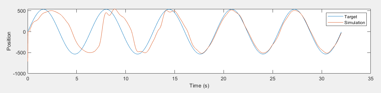
As I say, I will code up something more usable in python…
Yes, that sounds like a good idea!
In reply to Warren, your comment seems to be about public relations rather than about the science of PCT, except for one point:
What do you imply by “may or may not”? Are you saying that a prediction is either infinitely accurate or has no value as a prediction at all? If so, you totally missed the point of what I was saying. If not, what did you mean?
Let me try to put my main point in different (and I hope fewer) words. I trace a variation in the disturbance signal at time t0 around a single control loop.
-
When an environmental state registers at the sensors, a perception results. It has a value that for the sake of this argument we can incorrectly say exactly corresponds to the value of some environmental state (labelled the CEV, Corresponding Environmental Variable).
-
The control loop has both a discrete transport lag plus a distributed processing lag, the latter being non-zero only if the functions in the loop do some time-binding such as integration or differentiation. The processing lag is not a discrete value, but is distributed over time, in a decaying exponential if the output function is a leaky integrator.
-
By the time the transport lag has passed, and the very first effects of changes in the error value consequent on that initial perceptual value at time t0 have their effect on the CEV, the disturbance is likely to have moved on. Its current value is ∂t time units in the future of t0, the moment the sensory data were received. With an integrating output function, the strength of the output at time t0+∂t is increasingly affected by the old sensory input (at time t0) as ∂t increases. Time t0 was the moment the most recent observational data were available to the system.
-
The output at time t0+∂t opposes the disturbance at time t0+∂t with some error due to the amount the disturbance has changed during ∂t since the most recent available observation. For a continuously varying disturbance, that amount of change is captured in the autocorrelation function of the disturbance. It determines the minimum variance or uncertainty of the prediction looking ahead by a time ∂t, and it is therefore a limit on the best possible accuracy of control.
-
If the autocorrelation variance at future time ∂t equals or exceeds the long-term variance of the disturbance, the use of prediction produces worse results than ignoring it. Beyond the ∂t that produces equality, which I may call ∂tLIM, it is legitimate to say there is no effective prediction. At imes nearer in the future than ∂tLIM, prediction is potentially useful but is never perfect because of the transport and processing lags in the control loop.
-
In a control hierarchy, control is slower as one goes up the levels. For tracking, ∂tLIM may well be best measured in milliseconds. In politics, it is probably best measured in months or years if the measure is of preference rather than of elections that don’t happen and then do happen.
-
There is no sensible way of saying that perception (and memory) up to time t0 “may or may not” have predictive value at time t0+∂t based on whether a future observation at time t0+∂t is exactly a predicted value. Even if the prediction is of who will win an election, or some other event that a future observation will assign a discrete and exact value, the prediction is always of a probability distribution of the kind “Result X” has a probability of P(X) of being observed when the decisive event occurs. The prediction does not fail even if P(X) is 0.001 and X turns out to be the result afterwards.
-
From a Public relations viewpoint, none of the foregoing argument is at all relevant. The general public agreed that the pollsters in the 2016 US Presidential election got it wrong because most of them gave Clinton an 85% chance of winning, and she didn’t. The public relations problem with the word “prediction” is worth discussing, but not in this thread “Delay in control loops”.
Sorry, of course you are right that the accuracy of prediction can be on a sliding scale.
If only science were just about public relations! Unfortunately scientists reify and believe the terms they use, and they become solidified in the assumptions that hold back societal progress. Bill knew this and he wanted PCT to cut through it…
It is syncing pretty nicely!
As I say, I will code up something more usable in python…
Sure,it looks pretty wild, both memory and reorganization! Looking forward to it.
I’ll see if I can make a “target presentation and cursor recording” widget for a jupyter notebook. Maybe that would be good enough to make some trial recordings in colab.
Here is a start:
Jupyter notebook tracking task.
It is mixing some javascript and python to make the widget, it should work in local jupyter notebooks, or colab or mybinder.
Nice! The widget seems to work well!
I’ve followed your lead and made a colab thingy with the memory sine tracking thing:
It doesn’t seem to handle a large discrepancy between the initial condition for the sine frequency parameter and the actual sine frequency very well. This may just be due to the reorganisation algorithm as I’ve implemented it though - I have found reorganisation to be very temperamental and trying to improve the algorithm a bit.
The reorganisation system here doesn’t operate with a transport delay either, which is very implausible. As I said, I have a few problems with the reorganisation algorithm, but I’ll try to address these in another topic.
Update: I noticed some errors in this last script. A new version is much improved and is able to find the correct frequency much more quickly and much more often. This time it uses the error between the input function sinusoid and memory rather than control error as the reorganisation error term.
Cheers