No you did not answer, not well, not badly, not at all. You just repeat your credo again and again. Perhaps I must say this more clearly: Would you please answer these questions and with arguments, not just that you believe so:
a) Think (or make) a program which draws rectangular quadrangles and between every drawing it randomly changes the length of either the width or the height of the next quadrangle. (Hopefully this is understandable English!) Now, do you think that there is a mathematical dependence relationship between the width and height of this randomly changing quadrangle?
b) If you think that there is a mathematical dependence between the width and the height, do you think so because the area of these differently sized and formed quadrangles can be calculated from their current width and height with the eq. (7) of my previous message: A = W x H ?
c) If you think that there isn’t a mathematical dependence between the width and the height, then why there should be such relationship between the velocity and the curvature of a trajectory just because the D (a cube root of so called affine velocity) can be calculated with the eq. (6) from the velocity and the curvature?
Minor point. A behavioural illusion is perceived by the controller, whereas the curvature-velocity relation in any specific case has to be determined by a third-party analyst. So the power-law relation is not a behavioural illusion. It is an analytical fact, a side-effect of whatever the moving controller is controlling.
(My guess is the lateral acceleration that is equivalent to a lateral force that might exceed the traction of the moving entity. This force can be sensed by the moving entity, which makes it a candidate for being a controlled perception. But that’s just a guess.)
I guess “behavioural illusion” means different things to different people. I must say that I never thought about it before — or at least, not recently. As I had thought about it, Eetu is right, but it was a mistake on my part that led to an unnecessary side-track in the main discussion.
What I wanted to get across is that the power-law relationship frequently observed by analysts in different situations is not a controlled variable, but is a side-effect of whatever perceptual variables are controlled.
Right, it will be a side effect of control of any perceptual variable(s) as long as curved movements are required to control that variable. It will also be see in any curved movement whether that movement is part of a control loop or not. A mathematical characteristic of the relationship between V and R will always result in close to a 1/3 power relationship when R is regressed on V and D is left out of the analysis.
The power law is Boojam, not a Snark!! I just don’t want you guys to “softly and suddenly vanish away”.
I have been answering with arguments. There may be no way for me to help you to understand. But it’s fun trying so here we go.
I actually made a little spreadsheet just for you (well, actually, for everyone who wants to understand what’s going on) that does exactly what you ask. Download it and open in Excel.
The first three columns do what you ask, producing 100 rectangles of randomly varying height (H) and width (W). Each row in the columns is a different, randomly generated rectangle The first column is the area (A) and the 2nd and 3rd are H and W , respectively of the rectangle. I’ve made it possible to raise H to any exponent by entering a value into cell I1. The current value is 1 so that A = H * W.
You don’t need the spreadsheet to tell you that; no, there is no mathematical dependence between H and W. However there is a statistical (correlational) relationship between H and W as shown in cell I3, labeled r(H,W). I also show the correlation between the logs of H and W below that. Pressing key F9 generates 100 new rectangles with random values for H and W. This changes the correlation between H and W but, because they are statistically as well as mathematically independent the correlations are typically very small(<.2)
I don’t think there is a mathematical dependences between H and W.
This is why I made the spreadsheet. The equation for area,
A = H *W
is exactly analogous to the equation for velocity,
V = R^1/3*D^1/3
where the implicit exponents of 1 for H and W are analogous to the explicit exponents of 1/3 for R and D.
You ask “why there should be such relationship between the velocity and the curvature of a trajectory just because the D (a cube root of so called affine velocity) can be calculated with the eq. (6) from the velocity and the curvature?” The answer is that the relationship between velocity (V) and curvature (R) is not found because D can be calculated from the velocity and the curvature. It is found because V is mathematically related to R, just as a relationship between H and A will be found because A is mathematically related to H, not because W can be calculated from A and H.
The spreadsheet shows what you would find if you did a regression of just H on A, using the regression equation A = k+ BetaH, which is exactly analogous to what power law researchers are doing when they regress R on V. But since power law researchers are expecting a power relationship between R and V they regress log (R) on log (V) using the regression equation
log (V) = log(k) + Beta*log (R)
so the analogous regression for H on A is to regress log (H) on log (A) using the regression equation
log (A) = log(k) + BetaH*log (H).
The results of this regression are shown in cells H6 - J6 labeled BetaH, k and r2, respectively. BetaH is the estimate of the exponent of H in A = H * W, which is 1. k is the intercept constant and r2 is a measure of the goodness of fit of the regression equation.
As you can see by repeatedly pressing F9, the estimate of BetaH for different sets of 100 randomly generated rectangles varies around the true value, 1.0, occasionally being exactly 1.0 but usually deviating from 1.0 by as much as .15. The r2 for the fit is generally pretty poor, as one would expect, rarely getting above .3 but occasionally getting up around .68.
The results of the regression of log (H) on log (A) is exactly what is going on in power law research when researchers regress log (R) on log (V). They often get an estimate of Beta, the exponent of R in M&R equation (5), that is close to the true, mathematical value,1/3, but sometimes they get values that deviate from 1/3 by quite a bit.
Of course, we get the results we do from the regression of log(H) on log (A) because we have left out the other variable that we know determines the value of A, the width of the rectangle, W. When we include W in the regression we get an exact estimate of the true exponent of H, 1.0, as shown in H8. The regression equation used was
log (A) = log(k) + BetaHlog(H) + BetaW log (W)
and this regression always gets the exact, true value for both BetaH and BetaW, and the r2 is always 1.0.
You can run an even closer analogy to the situation with the power law by changing the setting the exponent of H in cell I1 to something other than 1.0 (that is greater than 0 and less than 1). If, for example, you set it to .33 then the equation for A becomes
A = (H^.33) * W
and you will see that the estimate of the exponent of H when log (H) is regressed on log (A) (in cell H6) is close to .33 rather than to 1, and the estimate of the exponent of H when regression includes both log (H) and log(W) (in cell H8) will give it’s exact true value, .33 in this case.
The degree to which the estimate of the coefficient of H will deviate from its true value (whatever was set in cell I1) can be calculated if one knows the value of the variable omitted from the analysis, which is the width variable, W. The deviation of the exponent observed in the regression of log (H) on log (A) from its true value is exactly equal to the covariance of log (H) with log (W) divided by the variance of log (H). That value is shown under the delta in cell K6. Notice that the value of delta shown in K6 shows exactly how much the value of BetaH in cell H6 deviates from the true value in I1.
I hope I have answered all your questions. But if not or if you have any trouble understanding what is going on in the spreadsheet and how what is being calculated in the spreadsheet is analogous to what is calculated by power law researchers feel free to ask.
Thank you Rick, it was nice and very kind that you made that spreadsheet. I hope it will help the continuation of the discussion. But I am sorry I cannot continue the discussion immediately, because of the conference of Finnish Educational Research Association here in Oulu in Thursday and Friday. I have there a presentation where I talk about basics of PCT and I now have to concentrate on finalizing it.
RM: I actually made a little spreadsheet just for you (well, actually, for everyone who wants to understand what’s going on) that does exactly what you ask. Download it and open in Excel.
Thanks again for that! Let’s see.
RM: You don’t need the spreadsheet to tell you that; no, there is no mathematical dependence between H and W. However there is a statistical (correlational) relationship between H and W as shown in cell I3, labeled r(H,W). I also show the correlation between the logs of H and W below that. Pressing key F9 generates 100 new rectangles with random values for H and W. This changes the correlation between H and W but, because they are statistically as well as mathematically independent the correlations are typically very small(<.2)
I am glad to read that. (Just a little note: I am used to a saying that if there is very low correlation between two variables and thus they are statistically independent then there is NO statistical relation between them, but that is only a way of talk. Anyway, also no relation is a relation.)
RM: This is why I made the spreadsheet. The equation for area,
A = H * W
is exactly analogous to the equation for velocity,
V = R^1/3 * D^1/3
where the implicit exponents of 1 for H and W are analogous to the explicit exponents of 1/3 for R and D.
No, not exactly! The order of the members is different. The “roles” of the members are different and the order should follow that. This is the critical core point! H and W as the multiplicands are basic measurements (or independent random numbers in this example) and A as a product is a higher level construct constructed from H and W. Similarly the velocity and the curvature are basic measurements which can be measured independently (even though they can both be constructed from the still more basic level measurements of x and y directional transition in a time unit, but the curvature can also be measured from the curved line drawn in the coordinates without any transitions bound in time) while D (or affine velocity or anything like them) is a higher level construct constructed as a product of curvature and velocity. So, the exact analogy of
A = H x W
is
D = V^3 x 1/R or
D = V^3 x C
RM: The answer is that the relationship between velocity (V) and curvature (R) is not found because D can be calculated from the velocity and the curvature. It is found because V is mathematically related to R, just as a relationship between H and A will be found because A is mathematically related to H, not because W can be calculated from A and H.
Here again you mix the places and roles of the variables in the equations. In a way H is mathematically related to A, because A is calculated from H and another variable, but this not any real mathematical relationship if we don’t take into account also the other multiplicand, W. However, understandably there is much stronger correlation between H and A than between H and W: about .5 – .7 But I did not ask about the relationship between H and A but between H and W. (Respectively, power law researchers are not interested in the relationship between curvature and D or between velocity and D but in the relationship between velocity and curvature.) The correlational relationship between H and A exists because and only because A is a product of H and W. And respectively correlational relationship between V and D exists because and only because D is a product of V^3 and C.
RM: The spreadsheet shows what you would find if you did a regression of just H on A, using the regression equation A = k+ BetaH, which is exactly analogous to what power law researchers are doing when they regress R on V. But since power law researchers are expecting a power relationship between R and V they regress log (R) on log (V) using the regression equation
log (V) = log(k) + Beta*log (R)
so the analogous regression for H on A is to regress log (H) on log (A) using the regression equation
log (A) = log(k) + BetaH*log (H).
The same confusion continues here. The analogous regression equation should be:
log (W) = log(k) + BetaH*log (H)
RM: The results of this regression are shown in cells H6 - J6 labeled BetaH, k and r2, respectively. BetaH is the estimate of the exponent of H in A = H * W, which is 1. k is the intercept constant and r2 is a measure of the goodness of fit of the regression equation.
As you can see by repeatedly pressing F9, the estimate of BetaH for different sets of 100 randomly generated rectangles varies around the true value, 1.0, occasionally being exactly 1.0 but usually deviating from 1.0 by as much as .15. The r2 for the fit is generally pretty poor, as one would expect, rarely getting above .3 but occasionally getting up around .68.
No, if you do that regression between H and W (analogously to power law research) you will get nothing like that. BetaH varies wildly between -0.1 and +0.1 (occasionally bigger). So there is no relationship and especially no “true value” of BetaH! The same is true also of any random curved trajectory.
RM: The results of the regression of log (H) on log (A) is exactly what is going on in power law research when researchers regress log (R) on log (V). They often get an estimate of Beta, the exponent of R in M&R equation (5), that is close to the true, mathematical value,1/3, but sometimes they get values that deviate from 1/3 by quite a bit.
As I have already said above at least twice, the relationship between H and A has nothing to do with the relationship between H and W. I have attached a little bit corrected spreadsheet and with it you can yourself learn that. Then after that I suggest another lesson: Change the titles of the columns so that A becomes D, H becomes V, and W becomes C.
Then when I ask you: Do you think there is a mathematical dependence relationship between the velocity and the curvature of a randomly changing curve? You should be able to answer also here that “no, there is no mathematical dependence between” V and C.
This is what it means that V = R^1/3*D^1/3 fits to every possible trajectory and every possible curve. It means the same that A = H x W fits to every possible rectangular quadrangles. Not only D = V^3 x C fits to every possible curve but as well fits E = V^2 x C ; F = V^4 x C ; G = V^5 x C; etc. etc.
I hope this is enough about the mathematical dependency relationship between the curvature and velocity?
Actually, there is a mathematical relationship between H and W. Since A = H*W the H = A/W and W = A/H. The same mathematical dependency exists for C and D in the equation for V. Since V = R^1/3 * D^1/3 then R = V^3/D and D = V^3/R
So D is equivalent to A, H to V and W to C. So the rectangle analogy to the power law equation
V = C^-1/3 * D^1/3
is
H = W^-1*A^1
since mathematically H = A/W. And the log-log regression equation is
log(H) = BetaW x log(W) + BetaA x log(A).
Where the true values of BetaW and BetaA are -1 and 1, respectively.
I’ve made a new spreadsheet so that the regression is done on log (W) predicting log (H), which I believe you are saying is the correct analog of what power law researchers are doing when they regress log(C) on log (V). The new spreadsheet is here.
What it shows (by comparing cell H6 to H10) is that if you regress log (W) on log (H) (the analog of regressing C on V) you end up with an estimate of a power coefficient, BetaW, that is not close to it’s true mathematical value (-1.0). However, if you include the covariate, log (A) in the analysis you find that BetaW is exactly -1.0 (and BetaA is 1.0).
The spreadsheet also shows that the deviation of BetaW (the analog of the power law coefficient) from its true mathematical value (-1 in this case) depends exactly on the covariance between log (W) (the analog of log (C) in power law analysis) and log (A) (the analog of log (D), the omitted variable in power law analysis). The predicted deviation is shown as the value of delta in cell K6.
That is fixed in this new spreadsheet where W is regressed on H rather than on A. And we get the same result. The observed power coefficient relating W to H deviates from the true value in proportion to the covariance (similar to correlation) between W and the omitted covariate, A.
In the new spreadsheet I regress W on H using the following:
log (H) = log(k) + BetaW x log (W)
This gives you the same results as if you had regressed H on W, as suggested by your equation. The result is that the power exponents of the predictor, BetaH in your equation, deviates from its true value (-1) by an amount, delta, that is proportional to the covariation between the included predictor, log (H) in your equation, and the omitted covariate, log (A).
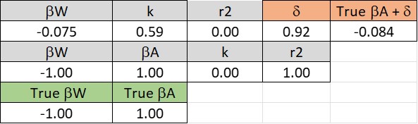
When you do the regression between only H and W you do get a value for the power coefficient that varies around 0. You only see the true value, -1, when you include the omitted covariate, A, in the analysis. This is shown in the spreadsheet table:
The table shows that when regressing W on H (omitting A) the observed power coefficient, BetaW, was .118 for this data set. But when the covariate, A, is included in the regression, BetaW is found to have it’s mathematically true value, -1.
As I have already said three times above;-) I have changed this “problem” in the new spreadsheet. And, of course, the results are the same as they were when A was used as the dependent variable. When H is regressed on W, or vice versa, the observed “power coefficient” deviates from it’s “true” mathematical value by an amount, delta, that is proportional to the covariance between the predictor variable (H or W) and the omitted variable, A.
Well, I’m afraid I’m unable to do that because the new spreadsheet shows that there is a mathematical dependence between H and W just as there is between V and C.
The new spreadsheet shows that that “meaning” is specious.
[If someone still tries to follow this discussion I try recap a little:
Rick has stated that it is vain waste of time to study a research question of why there is often found a special empirical relationship between the velocity and curvature in curved movement trajectories produced especially by living beings. (This relationship means coarsely that the velocity is slower if the curve is steeper.) He claims that curvature and velocity are mathematically related so that the often but not always empirically found relationship actually prevails in every possible curved movements. His founding argument is an equation according to which the curvature times the velocity to the power of three is a variable called D [D = V^3 x C]. (The value of D varies and depends on the values of the multiplicands.)
My (our) counter argument is that if the equation [D = V^3 x C] fits to all possible curved trajectories, as Rick confirms that it fits, then it fits to every possible pair of instantaneous values of velocity and curvature. From this follows that the instantaneous velocity and respective curvature can be set as randomly changing variables. Now the disagreement has boiled down to the question is there a mathematical dependence relationship between two random variables.]
Rick, it is almost admirable how fluently you contradict yourself – if it were not so bad thing for scientific discussion.
First you say that “no, there is no mathematical dependence between H and W” and then you say that “Actually, there is a mathematical relationship between H and W”. The explanation of this contradiction seems to be this: When you think about H and W as two separately set random variables you see clearly that they are not mathematically related. But when you start to think them as multiplicands of an equation [H x W = A] you start to think that they are mathematically related.
But regardless of any possible numeral operations between H and W they still remain those same separately and independently set random variables – and not mathematically related. Equations like [H x W = A] (and its equivalents like [H = A/W ]) cannot posit any dependency relationships between H and W.
This is the core of our disagreement and I think your position is quite desperate. Could you for example ask about it from a distinguished mathematician Richard Kennaway to whom I think you rely?
Thanks for a new spreadsheet. It is nice but there you fool yourself by a cheap sleight of hand: You change the original setting and now W and A are random variables and H is calculated as A/W. My original question was about mathematical relationship between two random variables. Of course there is a dependency relationship between two variables if only one of them is random and the other one is calculated from that random variable, but it is a totally different situation and question.
I’m sorry. On re-reading I realized that you were asking about mathematical dependence and, of course, there is such a dependence.
Actually, I’m learning that the degree to which these variables are stochastically independent can vary depending on the real world situation.
Actually, I don’t rely on Richard. He’s got much more important things to do.
The cheap slight of hand was not intended to deceive either of us. I calculated H from A and W (both random variables) because the regression gave results more like those found by power law researchers, as shown here:
This analysis is found in a sheet labeled “Constrained H DV” in the new version of the spreadsheet. Note that BetaW for the regression of log (W) on log(H) is -.944, which is very close to the true value, -1.00. This is because the covariance between log(W) and the omitted variable, log(A), is quite small so that delta – the deviation of the observed BetaW from the True BetaW due to omitting log (A) from the analysis – is also quite small. When the covariate, log(A), is included in the analysis, BetaW is found to have its true value, -1.0.
This is what is observed in power law research, where the observed Beta for curvature is close to .33, which is the true value of the Beta for curvature. This happens in power law research because the covariance between curvature and affine velocity is typically small for curved trajectories. So the deviation (delta) of the Beta for curvature from its true value is proportional to the covariance between curvature and the variable omitted from the regression, affine velocity, for that movement trajectory.
If both W and H are random variables, then you get results like this:
Now BetaW is -.075, which is close to zero. This is quite a large deviation from the true value of BetaW, which is -1.0. This deviation is accounted for (though not exactly, I don’t know why yet) by the large value of delta, which results from the large covariance between log (W) and the omitted covariate, log (A). When the covariate, log(A), is included in the analysis the observed estimate of BetaW is exactly equal to its True value, -1.
So thanks to doing the regression on the variables calculated in these two different ways, I have learned a lot about why a side effect of controlling for making curved movements is typically a power relationship between curvature and velocity with an exponent that rarely deviates by much from .33. Now I just have to figure out why the covariance between curvature and affine velocity in almost all curved movements is close to 0.0.
RM: I’m sorry. On re-reading I realized that you were asking about mathematical dependence and, of course, there is such a dependence.
Seems like you must be here thinking something else than me. With mathematical dependence relationship between two variables I mean a relationship where the value of the other, dependent, variable (say A) can be calculated by some mathematical equation from the value of the other, independent, variable (say B). The simplest this kind of dependence equation is that of identity:
[A = B]
Others can be like:
[A = k * B^l + m]
where k, l, and m are suitable constants.
During this discussion I have been thinking this kind of unconditional or exact dependence relationship, but now I see that the relationship can also different: conditional, loose, or fuzzy. In latter kind of cases it is not possible to calculate exactly the value of A from the value of B but still A’s value is affected by the value of B according to some mathematical equation. The simplest (and perhaps fuzziest) example is non-identity:
[A ≠ B]
Other examples could be such where there are more than two variables like in this:
[A = B * C]
Here B affects the value of A but does not determine it because also C is as strongly affecting it.
From a mathematical dependence ensues a stochastic dependence. In the case of exact dependence also the stochastic dependence is as strong as it can be, in linear cases correlation is ±1 with no exceptions. Respectively in fuzzier cases also the stochastic dependence is weaker. But common to all mathematical dependencies between A and B is that one of them must be independent and the one dependent. If they both are separately set random variables then they both are independent and so there cannot be any mathematical independence relationships between them.
RM: Actually, I’m learning that the degree to which these variables are stochastically independent can vary depending on the real world situation.
Yes, in the real world situations (or studies of them) the stochastic dependences usually vary if they do not ensue from mathematical dependencies. If a dependence is strong (correlation ±1) and stable then it is quite surely a sign that the dependence ensues from exact and tautological mathematical dependence, and thus result of the study does not tell anything about the real world but only about our mathematical conceptions. Between genuinely independent random variables there cannot be any mathematical dependence, so if a (reliably strong) stochastic dependence is empirically found then it must ensue from causal relationships – either between the variables or between both them and some third variable.
RM: Actually, I don’t rely on Richard. He’s got much more important things to do.
A wrong word choice, sorry. I meant that you possibly trust on Richards mathematical competence.
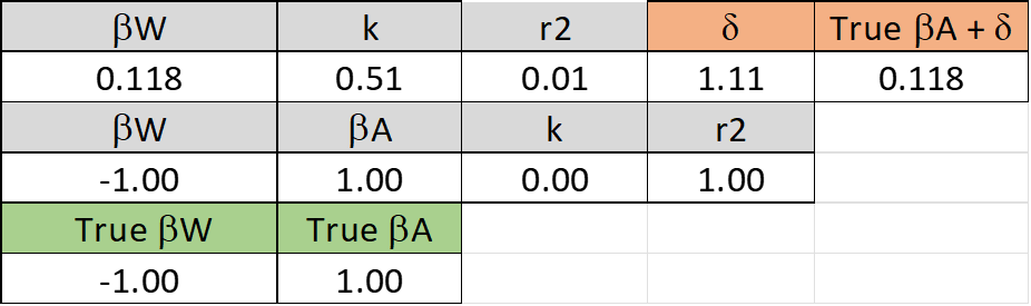
RM: The cheap slight of hand was not intended to deceive either of us. I calculated H from A and W (both random variables) because the regression gave results more like those found by power law researchers, as shown here:
[Picture1]
This analysis is found in a sheet labeled “Constrained H DV” in the new version of the spreadsheet.https://www.dropbox.com/s/jrzw0r465tmpgzq/For%20Eetu%203.xlsx?dl=0 Note that BetaW for the regression of log (W) on log(H) is -.944, which is very close to the true value, -1.00. This is because the covariance between log(W) and the omitted variable, log(A), is quite small so that delta – the deviation of the observed BetaW from the True BetaW due to omitting log (A) from the analysis – is also quite small. When then the covariate, log(A), is included in the analysis, BetaW is found to have its true value, -1.0.
No you can’t (or shouldn’t) arbitrarily change the situation so that you are no more studying the relationship between random variables H and W, but instead the relationship between three variables H,W, and A where now W and A are random and H is calculated from them. Now you yourself create there the mathematical relationship. Between random H and W there is no such relationship and thus there can be no “true” regression value between them: no dependence = no regression.
Once again, if H and W are mathematically independent separately set random variables, you cannot create a dependence relationship between them just by putting them to a numeral operation. That operation can be multiplication (X = H * W), addition (X = H + W), subtraction (X = h - W), power (X = H^W), or any. They all create different dependence between all the three X, H, and W together but none between H and W.
RM: This is what is observed in power law research, where the observed Beta for curvature is close to .33, which is the true value of the Beta for curvature. This happens in power law research because the covariance between curvature and affine velocity is typically small for curved trajectories. So the deviation (delta) of the Beta for curvature from its true value is proportional to the covariance between curvature and the variable omitted from the regression, affine velocity, for that movement trajectory.
In the case of quadrangles H and W affect both us much to the area A (A = H * W). That is why you get that beta between H and A is ±1. It follows from the form the numeral operation by which you yourself create the mathematical dependence between the three variables. In the case of D or affine velocity there is the inequality between the powers of velocity and curvature, because velocity is raised to the power of three in the equation (D = V^3 * C). That is why you will get the beta value ±1/3. The beta is literally constructed by you, a statistical artifact.
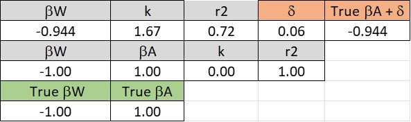
RM: If both W and H are random variables, then you get results like this:
[Picture2]
Now BetaW is -.075, which is close to zero. This is quite a large deviation from the true value of BetaW, which is -1.0. This deviation is accounted for (though not exactly, I don’t know why yet) by the large value of delta, which results from the large covariance between log(W) and the omitted covariate, log (A). When the covariate, log(A) is included in this analysis the observed estimate of BetaW is exactly equal to its True value, -1.
Zero is the true Beta value between independent random variables. -1 is untrue, fabricated value, which you create by selecting the form of the equation between the original two variables and a third extra variable.
RM: So thanks to doing the regression on the variables calculated in these two different ways I have learned a lot about why a side effect of controlling for making curved movements is typically a power relationship between curvature and velocity with an exponents that rarely deviates by much from .33. Now I just have to figure out why the covariance between curvature and affine velocity in almost all curved movements is close to 0.0.
I think you can easily figure it out empirically from different trajectories. I bet you will find that always when the 1/3 power law is obeyed the affine velocity (and D) is stable. There is such a dependence relationship that if one variable varies and the other remains stable then there is no covariance. But this result does not explain why there sometimes is covariance and the trajectory does not obey the power law. That is the original research question of power law researchers turned just around.
I still cannot access the Discourse web interface.
The message below became malformed by Discourse so that in the end side the paragraph below was formed as a quotation even though it was written by me there:
In the case of quadrangles, H and W affect both us much the area A (A = H * W). That is why you get that beta between H and A is ±1. It follows from the form the numeral operation by which you yourself create the mathematical dependence between the three variables. In the case of D or affine velocity there is the inequality between the powers of velocity and curvature, because velocity is raised to the power of three in the equation (D = V^3 * C). That is why you will get the beta value ±1/3. That beta is literally constructed by you, a statistical artifact.
Sorry to reply again to my own message but I forgot to add an important conclusion to it.
In the spreadsheet there are two random variables in the columns A and B (called H and W). Then in the third column C there is an extra variable which is calculated from the first two variables by an equation HW. In the first spreadsheet the columns were in a different order which does not mean anything but there was in a handy way the equation written as H^ExpW and you could change the exponent Exp in a special cell (L1) of the spreadsheet. So if you write 1 to the L1 cell then the equation for the extra variable would be just HW which is the equation of an area of a quadrangle, but if you write there 3 then the extra variable would be D: V^3C.
Note that the values in the columns A and B need not change even if the exponent Exp and the names of the columns were changed – and it would not matter even if they were changed because they are only pure random numbers. The values in the columns A and B represent the sides of a random quadrangle if they are named H and V and Exp is 1. If Exp is 3 and the names of the columns are V and C then they represent the velocities and curvatures of a random trajectory. Just the same data could describe and fit to both phenomena and any other random value pairs.
Now, utilizing the Omitted Variable Bias method invented by Rick we can find as many different “true” dependency relationship descriptors (Beta values) between two independent variables in the same data as we want to. Is this kind of research method useful? Yes it is if you want to prove true something which is not true.
Some kind of bug in the current update of Discourse is preventing some users from accessing Discourse, and Rick is one of these. I don’t know if it’s the user’s computer platform (Rick uses a Mac) or the browser (Rick is probably using the Mac default, Safari) or something else. In any case, there is a delay before he can respond to any of this.
Well, Eetu, if the spreadsheet doesn’t convince you that the power law is a statistical artifact – a side effect of control that is explained by how researchers have measured it – then I will no longer try to prevent you and your hunting party from stalking that Boojam. l’ll just note that I can’t claim credit for inventing Omitted Variable Bias (OVB) analysis. This tool, which you believe is used “to prove true something which is not true,” was “invented” some time ago by others. And though it was not called by that name, OVB is the analysis of the power law that was described by Moaz et al (2006) well before I descsribed it in Marken & Shaffer (2017).
I realize any discussion of the Power Law effect is fruitless, but perhaps it is worth letting others know that Moaz et al. (2006) did not make the mistake that is the heart of the problem with Marken and Shaffer (2017). There’s no point in restating the Marken-Shaffer mistake for the Nth time. Its been shown by several people in several different ways.