Economic Data Analysis

Economic Data Analysis
[From Rick Marken (2004.02.04.1025)]

Here are some more data analyses that I did some time ago to test some popularly held ideas about how the economy works. One such idea is that the Fed discount rate can be used to control inflation. The discount rate is used to influence the amount of money in circulation. Increasing this rate takes money out of circulation.

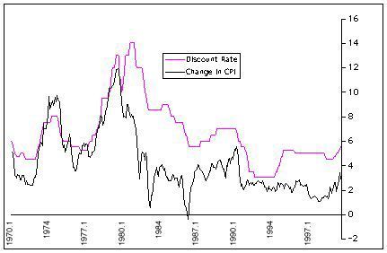
Apparently under the theory that inflation results from too much money in circulation, many economic policy makers believe that the Fed can tame inflation by raising the discount rate. A couple of years ago I went to the FRED data site and got the discount rate and CPI (consumer price index) data that was available. What I got was monthly measures of these two variables from 11/1970 to 5/2000, 354 data points. I derived inflation rate from the monthly CPI values and found the results shown in the inflatedisc.jpg attached. The result shows what appears to be a clear positive relationship between discount rate and inflation rate, exactly the opposite of the relationship assumed in popular discussions of economic policy.

[insert inflatedisc.jpg here]

image16.jpg

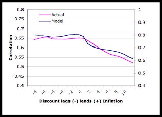
The positive relationship between discount rate and inflation rate shows up at nearly all phase delays between these time plots of these two variables. This is shown in the lagged analysis in the attached laginflatedisc.jpg. The lags/leads on the X axis are the number of months by which the discount rate leads (- values) or lags (+ values) inflation rate. Discount rate does not become negatively related to inflation until 22 months before the inflation changes. And the negative relationship is quite low. The negative relationship between discount rate and inflation never exceeds -.11, and that that level of negative relationship doesn’t occur until discount rate leads inflation by 36 months (3 years). Compare this to the very strong positive relationship (.59) between discount and inflation rate that reaches a maximum when discount rate follows inflation rate within 11 months.

[insert laginflatedisc.jpg here]

image17.jpg

The results of this analysis suggest, to me, that discount rate may be controlled (the control system doing the controlling being Greenspan) relative to inflation rate in a positive feedback control loop. That is, it look like Greenspan (or whoever the Fed chairman is) raises rates when inflation goes up and decreases rates when inflation goes down. This results in the positive correlation between discount and feedback when discount follows inflation (positive lag values). But changes in the discount rate seem to be positively related to inflation (rather than negatively, as assumed by the Fed) as indicated by the positive relationship between discount and inflation when discount precedes inflation (negative lag values). This positive feedback relationship between the Fed chief’s actions and the results of those actions on the controlled variable – inflation – would result in runaway inflation if the Fed chie kept raising rates. But the positive relationship between the Fed chief actions and inflation seems to level off after a few months. So runaway inflation is prevented by the limit to the Fed chief response to the inflation he has coaused causes by his own actions.

I think that’s the correct interpretation of the results in laginflatedisc.jpg. But I will run some simulations to check it out.

By the way, after producing the graph in inflatedisc.jpg from the raw data I found exactly the same graph in Canterbery, E. R. (2000) Wall street capitalism, River Edge: NJ, World Scientific. Canterbery’s book was pointed out to me because it makes considerable reference to the work of TCP. Anyway, if you get the book you will see that his Figure 14.1 (p. 266) is exactly equivalent to the graph I made that is shown in inflatedisc.jpg. And Canterbery comes to the same conclusion as I do about it: the observed relationship between discount rate and inflation is exactly the opposite of what many economic policy experts think it is.

Canterbury also looked at the relationship between Fed discount rate and economic growth. He presents his results in Figure 14.2, p. 269. That graph looks about the same as the one in growdisc.jpg, attached below.

[insert growdisc.jpg here]

image18.jpg

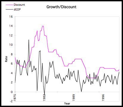
Apparently based on the visual appearance of this graph, Canterbery concluded that there is a negative relationship between discount rate and growth, which is, again, the relationship that is believed to exist between discount rate and growth by many economic policy experts. Increases in the Fed discount rate takes money out of the economy, which should make it difficult to get money for investment and growth. My own visual inspection of the data led me to the same conclusion: it looks like discount rate and growth are negatively related. But I wanted a quantitative measure so I got the raw data and made my own version of Canterbury’s Figure 14.2, which is the graph is seen in growdisc.jpg. I used the raw data (actually, I was able to get data that went back to 1959, rather than just 1975, but the statistical results are the same for the 1959-2000 and for the 1975-2000 time period) to compute the actual correlation between discount rate and growth. And the results were a big surprise. It turns out that the zero lagged correlation between discount and growth is positive (.25). The apparent negative relationship between the discount and growth curves seen in growdisc.jpg is actually an optical illusion. The complete phase analysis of the relationship between discount and growth is shown in the graph in laggrowthdisc.jpg.

[insert laggrowdisc.jpg here]

image19.jpg

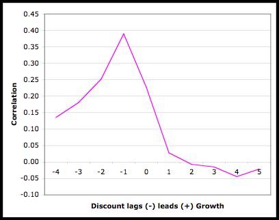
What this analysis shows is that changes in discount rate that precede growth are actually positively related to growth, a result that is, again, completely the opposite of what many economic policy experts seem to believe is true. Increases in discount rate are believed to lead to decreased growth. This would show up as a negative relationship between discount rate and growth when discount rate precedes growth. In fact, just the opposite is seen.

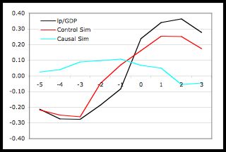
All the results presented here describe relationships between variables that exist as part of a closed loop system. I think the only way to figure out what is actually going on – that is, to figure out how variables like discount rate, grwoth and inflation actually influence each other – is to build closed loop models and try to match the behavior of the models (over time) to the observed behavior of the variables observed.

Best

Rick

···

Richard S. Marken

MindReadings.com

Home: 310 474 0313

Cell: 310 729 1400

[From Bill Powers (2004.02.04.1219 MST)]

[From Rick
Marken (2004.02.04.1025)]

Here are some more data analyses that I did some time ago to test some
popularly held ideas about how the economy works. One such idea is that
the Fed discount rate can be used to control inflation. The discount rate
is used to influence the amount of money in circulation. Increasing this
rate takes money out of circulation.

Good careful work, Rick. I like the way you check things rather than
taking them for granted – for example, that changing the number of years
of data used does not affect the result.

This is building up a nice backlog of studies of the data base. Keep all
these things handy. I can see a collaborative paper in the not-so-distant
future, led by a genuine economist, but strongly based in PCT.

I’m reading Charlotte Bruun’s thesis, in particular the chapter on Money,
and learning a lot. One thing I have learned from her is that TCP was
quite correct in saying that the composite producer simply created money
when it was needed. His rationale, as I recall, was that the banking
system is simply part of the composite producer, the part performing the
service of creating and storing money, and charging a fee for doing so.
This idea was taken by some as a sign of his senility, but apparently
it’s a well-recognized position that exists in some economic schools. The
creation of money by lending is apparently the correct view. There are
arguments about the “role” of money, but the possible roles are
apparently about classification schemes, and have no objective effect on
how money is actually used. The main effects would appear to be
subjective, and thus to be made part of the models of agents.

Bruun sees the need to keep track of physical aspects of the system
separately from the monetary aspects. For example, she said that if it
takes 1.2 KG of iron and three hours of labor to make a piece of capital
equipment, that is how it should be recorded, not in terms of the cost in
money. The cost can change, but it will still take the same amount or
iron and labor to make the part. I have written to ask why this should
not apply to consumer goods as well (as it does in Econ004C).

Bruun also concludes that it is necessary to conceive of the agents in
the economic system as purposive, rather than as rational (driven by
logic). Good things lie ahead, I think.

By the way, an average leakage rate of 7.5% would be accounted for if
loans were repaid at the rate of 7.5% of the outstanding principle each
year. Repaying loans destroys money. That’s not quite right, because
money is transformed from “credit” (repayable) into
“currency” (permanently circulating) when loans are defaulted
and the bank writes off a loan. So there has to be a certain relationship
between defaulting on loans and repaying loans to account for the 7.5%
average amount of leakage (called “savings” by
some)…

Best,

Bill P.

[From Bill Williams 4 February 2004 2:10 PM CST]

[From Bill Powers (2004.02.04.1219 MST)]

        [From Rick Marken (2004.02.04.1025)]
  
        Here are some more data analyses that I did some time ago to test some popularly held ideas about how the economy works. One such idea is that the Fed discount rate can be used to control inflation. The discount rate is used to influence the amount of money in circulation. Increasing this rate takes money out of circulation.

Good careful work, Rick. I like the way you check things rather than taking them for granted -- for example, that changing the number of years of data used does not affect the result.

This is building up a nice backlog of studies of the data base. Keep all these things handy. I can see a collaborative paper in the not-so-distant future, led by a genuine economist, but strongly based in PCT.

I'm reading Charlotte Bruun's thesis, in particular the chapter on Money, and learning a lot. One thing I have learned from her is that TCP was quite correct in saying that the composite producer simply created money when it was needed. His rationale, as I recall, was that the banking system is simply part of the composite producer, the part performing the service of creating and storing money, and charging a fee for doing so. This idea was taken by some as a sign of his senility,

# Who ever said such a thing? I hope this isn't just a more subtle, don't fuck anymore pigs argument.

but apparently it's a well-recognized position that exists in some economic schools. The creation of money by lending is apparently the correct view.

# There are also things call printing presses that create what somepeople call high power money.

There are arguments about the "role" of money, but the possible roles are apparently about classification schemes,

# And, causal relations as well.

and have no objective effect on how money is actually used. The main effects would appear to be subjective, and thus to be made part of the models of agents.

# More people I think would describe money in terms of institutional and cultural arrangments rather than in
  terms of agency.

Bruun sees the need to keep track of physical aspects of the system separately from the monetary aspects. For example, she said that if it takes 1.2 KG of iron and three hours of labor to make a piece of capital equipment, that is how it should be recorded, not in terms of the cost in money.

# You almost surely are reading this out of context. The bills after all are payed in money-- which is what the money is for.

The cost can change, but it will still take the same amount or iron and labor to make the part. I have written to ask why this should not apply to consumer goods as well (as it does in Econ004C).

Bruun also concludes that it is necessary to conceive of the agents in the economic system as purposive, rather than as rational (driven by logic). Good things lie ahead, I think.

# A disjunctive distinction between "purposive" and "logical" isn't altogether unfamiliar, but it isn't neccesary
  either.

By the way, an average leakage rate of 7.5% would be accounted for if loans were repaid at the rate of 7.5% of the outstanding principle each year. Repaying loans destroys money. That's not quite right, because money is transformed from "credit" (repayable) into "currency" (permanently circulating) when loans are defaulted and the bank writes off a loan.

# Bank loans are commonly _made_ in terms of credit ballances, so I don't see where the new currency
  is coming from. Ordinarily, only a state treasury creates currency. You have this confused.

So there has to be a certain relationship between defaulting on loans and repaying loans to account for the 7.5% average amount of leakage (called "savings" by some)..

# About a million conventional economics students a year are the "some."

Maybe Rick could knock another myth in the ditch by checking to see what connection exists between the
rate of interest and inflation. and changes in the rate of interest and inflation, and changes in the rate of inflation.

Bill Williams

[From Rick Marken (2004.02.05.1100)]

Bill Powers (2004.02.04.1219 MST)--

This is building up a nice backlog of studies of the data base. Keep all these
things handy. I can see a collaborative paper in the not-so-distant future,
led by a genuine economist, but strongly based in PCT.

Will do, of course. Though it's kind of surprising that "genuine economists"
have not already discovered what I have discovered in these readily
available pubic data sources. Or it least it seems like they haven't.
Canterbery is the only "genuine economist" I know of, for example, who has
pointed out that variations in the Fed funds rate are positively rather than
negatively related to variations in inflation rate.

Best regards

Rick

···

--
Richard S. Marken
MindReadings.com
Home: 310 474 0313
Cell: 310 729 1400

[From Bill Powers (2004.02.05.1228 MST)]

Rick Marken (2004.02.05.1100)--

Will do, of course. Though it's kind of surprising that "genuine economists"
have not already discovered what I have discovered in these readily
available pubic data sources.

Are you reading Bruun's doctoral thesis? I think it suggests a sort of
answer to your comment, in the sense that economists have been mostly
concerned with abstractions. One of the huge problems seems to be saying
what "value" is -- what determines it, how you measure it, and so on. This
is very much like behaviorists trying to find what is reinforcing about a
reinforcer, or why a given stimulus has the "stimulus value" it has.
They're looking for an objective definition of value that can be given
apart from the human agents in the system. I am hoping that when Bruun
learns the concept of the reference level, it will offer some answers to
these questions that have not been considered in economics.

I have the tracking program (Delphi) automatically evaluating all four
parameters now, and I have changed the model:

procedure runmodel;
var t: integer;
     force,mass: double;
begin
  fillchar(delaybuffer,sizeof(delaybuffer),0);
  damping := 0.1*Dampset; // entries from screen buttons and tools.
  gain := 0.1*gainset;
  timelag := round(delayset);
  modelref := round(refset/10);
  mhand := hand[0];
  mhandvel := 0;
  mcurs := mhand;
  t := 0;
  mass := 0.1; // more like moment of inertia, kg-m^2
  while t < numentries - 1 do // 3600 entries.
  begin
   mperc := mcurs - targ[t];
   mdelp := transportlag(mperc,timelag); // delayed perception
   merr := modelref - mdelp;
   if merr > 1000 then merr := 1000
   else
   if merr < -1000 then merr := -1000;
   force := gain*merr - damping*mhandvel; // output is a force prop to error
   mhandvel := mhandvel + force/mass*dt; // velocity = integral(force/mass)
   mhand := mhand + mhandvel*dt; // position = integral(velocity)
   mcurs := mhand;
   modelpercep[t] := mperc; // store data
   modeldelperc[t] := mdelp;
   modelcursor[t] := mcurs;
   modelhandle[t] := mhand;
   fiterr[t] := mhand - hand[t]; // save diff between mod & real
hand
   inc(t);
  end;
end;

This is a model with position and velocity feedback and a load that has
mass. I think it comes a little closer than the other model with only
position feedback and no mass. Needs work, though. Delphi source attached
for those who want to try it.

I am also trying to port the Crowd program into Delphi. Many things have to
be done differently, but eventually all programs will have to be converted.
I discovered that my Turbo P version of Econ004 will not run under Windows
2000 on Mary's machine. The display goes nuts when the program sets the
screenet to 800 x 600, and runs for only a short time at 640 x 480, even
after I installed TP7 on that machine and recompiled everything. I assume
that no other DOS-based programs will run, either.

Best,

Bill P.

TrkAn2.pas (9.61 KB)

PurstrkAn.dpr (220 Bytes)

TrkAn2.dfm (4.47 KB)

Analyze2.pas (6.11 KB)

[From Bill Williams 5 Feburary 2004 3:10 PM CST]

Today, at the library I encountered the following review.

_The Economic Process: An Instantaneous Non-Newtonian
Picture_. By Carmine Georga. Lanham, MD, and Oxford
University Press of American. 2OO2. Pp xiv, 374. $69.OO.
ISBN 00-7618-2156-2. JEL 2OO2-1336
   This book is dedicated to the author's mentor, Franco
Modigliani and his teacher, Robert Mundell. With such a
pedigree behind the author's analysis, one expects a
substantial, interesting contribution to the development
of economic theory. The author claims that this book
will transform mainstream "economic theory into
Concordian economics...[where] mainstream economics
disappears as the linear, static 'dismal science of text
books and is replaced by an organic and dynamic structure
capable of responding to the daily needs of concrete
human beings.
  The book is divided into five parts.

[I will dispense with the reviewers description and skip ]
[ to a description of the modifications of the Keynesian ]
[ equations which Georga introduces ]

   With these unusual definitions, the author takes usual
Keynesian identities of Y = C + I; S = Y - C; and I = S;
and presents the Concordian version of them in terms of his
definition of them in terms of his definitions of S (savings)
and C (consumption) as follows;

Y = C + S;
I = Y - S;
I = C.

   Later in the analysis, the last two equations are converted
D is the distrabution of ownership rights.
   From these defintions some of the more bizarre statements
(conclusions) of the author are
   (1) "Investment has become something that is nonproductive."
           (p. 48.);
   (2) "Mainstream economic theory compels us to assert that
           the dollar bills in a safe deposit box, unused land,
           stockpiles of raw materials that are not needed in
           the immeadiate future, contrary to all reality are
           items that produce wealth" (p.49.)
    (3) ....
    ...
    ...
    (6) "There are so many broad ramifications ..[of this
            concordian model] that they can neither be
            analyzed nor listed in this book." (p. 193.)

   I believe these statements give the reader a flavor for
what is contained here.
   What is a reviewer to say about this Concordian "revolution"
when the author utilizes economic terms to mean different things
than is commonly accepted terminology by economists? Perhaps I
can utilize a passage from Keynes's review of Hayek's book
(The Pure Theory of Money: a reply to Dr. Hayek." Economica
(1931), reprinted in Donald E. Moggridge, ed. 1973, _The
Collected Writtings of John Maynard Keynes, XIII, London;
MacMillian, pp. 252) to express my judgment:
   "The book as it stands, seems to be one of the most frightful
muddles I have ever read, with scarcely a sound proposition in
it. It is an extraordinary example of how, starting with a
mistake [here substitute unusual definitions for mistake], a
remoreseless logician can end up in Bedlam."

            Paul Davidson
            Professor Emeritus, University of Tennessee

Professor Davidson has been the editor of "The Post-Keynesian
Journal of Economics since its founding.

Davidson's review appears in

The Journal of Economic Literature, Volume 41 ( December 2OO3)
p. 1284-5.

Bill Williams

···

to: I = H and P = D, where H is hoarding, P is production, and

[From Rick Marken (2004.02.06.0830)]

Bill Powers (2004.02.05.1228 MST)]

Rick Marken (2004.02.05.1100)--

Will do, of course. Though it's kind of surprising that "genuine economists"
have not already discovered what I have discovered in these readily
available pubic data sources.

Are you reading Bruun's doctoral thesis?

No. I downloaded a paper called "Growth and inequality in agent-based
models: effects of introducing a wealth tax". That was some time ago. It's
hard to tell what her model is from that paper. But it does seem like she's
taking an approach that is like the one you are suggesting. I guess the
paper I have to get is Bruun (1999) "Agent-based Keynesian economics:
Simulating a monetary production system bottom up". Is that her thesis?

Ah, I just found that paper on the web and downloaded it (the internet is
such a great database it almost makes up for its failure as a discussion
forum).

I'll get back to you as soon as I've had a chance to read about the Bruun
model.

Best regards

Rick

···

--
Richard S. Marken
MindReadings.com
Home: 310 474 0313
Cell: 310 729 1400

[From Rick Marken (2004.02.07.2330)]

I did some rather simple modeling in order to make sense of the lagged
correlation data I presented earlier. First, I looked at the the
lagged data on the relationship between discount rate and inflation. I
used a model that assumes that the Fed board (which votes on increases
and decreases in the discount or funds rate) is a control system that
is simply matching variations in inflation rate with its own variations
in discount rate. The variations in discount rate are assumed to have
no effect at all on inflation rate. The model is as follows:

p = Discount in preceding month-Actual inflation rate in the preceding
month

Discount = Discount + 0.1 * ((0.01 * (0-p)) - Discount) *dt, where dt =
1 month

The actual inflation rate is the monthly inflation rate based on the
CPI (consumer price index) data from the Department of Commerce . The
model assumes that discount rate has no effect at all on inflation
rate. The Fed board control system controls p, the difference between
the independently varying inflation rate and its own discount rate. In
other words, the model assumes that the Fed board is performing a
pursuit tracking task with the observed (actual) inflation rate as the
target and the discount rate as the cursor.

The fit of this simple model to the actual lagged correlation data is
shown below. The slow and gain parameters (.1 and .01, respectively) as
well as the one month lag (p is the perceived difference between
inflation rate and discount rate from the preceding month) are those
that gave the best visual fit of model to data.

The fit of model to actual data seems extremely good. The general
shapes and elevation of the lagged correlation curves for the actual
and model data are very similar. The fit would presumably be even
better if the actual inflation rate values used were the same as those
seen by the Fed board at the time. The CPI (and thus, inflation rate
data) are, of course, revised regularly. So the inflation rate in the
2003 FRED data base for June of 1974, for example, is not the same as
the rate as it was measured in July, 1974.

I used essentially the same kind of control model to understand the
lagged correlations between gross private investment and growth rate.
The model assumes that the aggregate producer is a control system that
adjusts current investment to match perceived demand. Perceived demand
is based on past GDP. The model is as follows:

p = ( Investment 4 quarters earlier - GDP 4 quarters earlier)
Investment = Investment + 0.001 * (300 * (0-p) - Investment) *dt, where
dt = 1 quarter

Again, the model assumes that the aggregate producer is doing a pursuit
tracking task, trying to match Investment to the moving target of
demand, GDP. The model that fits the data best assumes that the amount
to be invested depends on the difference between investment and GDP 1
year (4 quarters) ago.

The fit of the model to data (with best fitting parameters as shown in
the equations above) is shown below. The black sigmoid shaped curve is
the actual lagged correlation between lp/GDP (gross private investment)
and growth rate. The red sigmoid curve is the lagged correlation
between model output (divided by GDP, so that the model output is
Investment/GDP) and growth rate.

The fit of model to data is again rather good. The height and shape of
the actual and model lagged correlation curves are very similar. In
this case, the fit of the model would probably not be made better if
the GDP measures seen at the time were used because it's unlikely that
producers use GDP as their basis for controlling future investment (as
the model assumes). GDP is just a surrogate for the aggregate demand
perceived by the producers, demand which is probably perceived in the
form of orders for goods and services.

The model says that the aggregate producer allocates current investment
based on its memory of what was happening one year ago. The one year
lag in the model may represent the time it takes to perceive demand
based on orders and to go through the steps needed to make the
investment to increase productoin. But the result for the control
model make a pretty convincing case for the notion that investment is
controlled relative to perceived demand for what is produced.

I compared this control model of the aggregate producer with a simple
causal model, which assumes that current GDP is caused by prior
investment:

Investment 4 quarters earlier = 0.9 * Present GDP

The lagged correlation results for this causal model are shown by the
blue line (the Investment output of this model was again divided by
GDP). The lagged correlation for the causal model is always pretty
much the same regardless of the lag (I show the results for a 4 quarter
lag because that's what worked best for the control model, but the
results are the causal model are the same for all lags) and effect size
coefficient (the coefficient shown, .9, assumes a moderately strong
dependence of Present GDP on prior Investment).

Best regards

Rick

GrowthInvest.jpg

InflationDiscount.jpg

···

---
Richard S. Marken
marken@mindreadings.com
Home 310 474-0313
Cell 310 729-1400

[From
Bjorn Simonsen (2004.02.08, 08:50 EuST)]

[From
Rick Marken (2004.02.04.1025)]

What
I got was monthly measures of these two variables from 11/1970 to 5/2000, 354
data

points. I derived inflation rate from the monthly CPI values and found the
results shown in the

Inflatedisc.jpg attached.

Your
black graph is Change in CPI. How
many months are the change calculated for in
the graph
?

Which
is the denomination for your Y axis?

The
result shows what appears to be a clear positive relationship between
discount rate

and
inflation rate, exactly the opposite of the relationship assumed in popular
discussions of

economic
policy.

Is
it more correct to say …….between
the Change in discount rate and
the inflation rate,………….?

bjorn

The model is
as follows:

p = Discount
in preceding month-Actual inflation rate in the preceding

month

Discount =
Discount + 0.1 * ((0.01 * (0-p)) - Discount) *dt, where dt =

1 month

You are presenting us (me) an interesting
argumentation. I need to hear from you if I understand your formula as you.

For myself

Discount (t+1) = Discount (t) + 0.1*((0.01*(0-p) – Discount
(t))*dt, where dt = 1 month an P = Discount in preceding month – Actual inflation
rate in the preceding month.

Your Reference is 0, and the argument for that is that
you think:

The variations in discount rate are
assumed to have no effect at all on inflation rate.

It means that
you expect a perception where “Discount in preceding month-Actual inflation
rate in the preceding month = 0

Here I have a
problem because CPI is about 184 and the discount is nearly 1 (I think). I
guess you recalculate the Discount in preceding month and the Actual inflation
rate to something I don’t know. Please help me.

I think PCT, and
in the input function there is a conversion of the feedback signal and Disturbances.
It is easy to understand the conversion of a perceptual variable to a perceptual
signal, but I have problems with the conversion of the Discount in a preceding
month and the Actual inflation rate in a preceding

Month. The denominations
are so different. I think they estimate the CPI from the price of certain goods
and services relative to the price in a standard year in percent. And this estimation is in the method of
calculation independent of the discount.

You see I have a
problem.

I have confidence
to the way you think and I whish to learn more.

bjorn

···

From Bjorn
Simonsen (2004.02.08,16:15 EuST)]]

From Rick Marken
(2004.02.07.2330)]

Discount =
Discount + 0.1 * ((0.01 * (0-p)) - Discount) *dt, where dt =

1 month

And from your attachment

The slow and
gain parameters (.1 and .01, respectively) as

well as the
one month lag (p is the perceived difference between

inflation
rate and discount rate from the preceding month) are those

that gave
the best visual fit of model to data.

It is OK that “……are
those that gave the best visual fit of model to data.”

When we talk
about PCT, the gain and the slowing factor are explainable. I think Bill gave a
good explanation for gain in BCP and I think you gave a good account in your “Spreadsheet
analysis of …” where you wrote “The integration performed in real nervous
systems is not perfect; there is some loss or “leakage” from the integrator
over time. The leakage is captured by the loss due to slowing in the equation
for the output function.”

The Slowing
factor also explains how the higher levels accumulate outputs more slowly than
the lower level systems.

But simulating
the Discount here is just one level. How shall we explain the Slowing factor in
a logical way as regards the Discount?

bjorn

[From Bill Powers (2004.02.08.0734 MST)]

Rick Marken (2004.02.07.2330)--

I did some rather simple modeling in order to make sense of the lagged
correlation data I presented earlier. First, I looked at the the
lagged data on the relationship between discount rate and inflation.
I used a model that assumes that the Fed board (which votes on increases
and decreases in the discount or funds rate) is a control system that
is simply matching variations in inflation rate with its own variations
in discount rate.

This would mean that it's matching d(Discount)/dt to dp/dt.(variations). I
don't think that's what you mean.

  The variations in discount rate are assumed to have
no effect at all on inflation rate.

In other words, there are no feedback effects? How does the control system
work, then?

The model is as follows:

p = Discount in preceding month-Actual inflation rate in the preceding
month

Discount = Discount + 0.1 * ((0.01 * (0-p)) - Discount) *dt, where dt =
1 month

I'm totally confused. What are you modeling? You're saying that the
discount rate in the new month is a smoothed version of one percent of the
difference between negative discount rate (percent interest on loans) and
inflation rate (percent increase in prices relative to base year) for the
previous month. What does this represent? And why does the data plot show a
correlation plotted against a lag that goes from -10 to +10 units (years?
Months?).Is the correlation the controlled variable? Where is the plot of
discount rate or inflation rate?

Let f = inflation rate
     d = discount rate
     p = perception

we have
     p(t) = d(t) - f(t)

     d(t+1) = d(t) + 0.1* 0.01*(0 - p) - d(t)] or

     d(t+1) = d(t) + 0.1*(-0.01(d(t) - f(t)) - d(t)] or

     d(t+1) = d(t) + 0.1*(-f(t) - 1.01*d(t))

I think something got screwed up in your equations here. Is that 0.01 a
gain, or a conversion from percent (5) to fraction (0.05)? And why do we
end up subtracting both the discount rate and the inflation rate inside the
parentheses? I think you had better avoid drawing conclusions until the
model makes sense.

Best,

Bill P.

[From Bill Williams 8 February 2004 1:30 PM CST]

[From Bill Powers (2004.02.08.0734 MST)]

Rick Marken (2004.02.07.2330)--

>I did some rather simple modeling in order to make sense of the lagged
>correlation data I presented earlier. >

A more accurate description of what Rick is doing is not _modeling_ but
_data mining_. What it amounts to is a process of randomly specifying
relationships until a correlation emerges. If enough effort is expended
some very nice, nice looking that is, correlations can emerge. Do these
nice correlations have any causal signficance? Well, they might-- by
accident correspond to causal relationships, but it is unlikely that in any
particular case that they will actually do so. An associate here James
Webb and Peach published a paper in the Journal of Economic Issues
a number of years ago, on "Randomly Specified Models" You can
retrieve the reference using the AFEE webb site.

I have never actually seen the process of data mining and randomly
sorting to find a coorelation more clearly illustrated than by Rick's
reports.

This sort of thing just gets in the way, because, if it is taken seriously
you have to put forth the effort to find the errors before you can get back
to real work. For this reason, this sort of stuff is prohibited by those I
know who do econometrics. See my previous posts and the reference
to the paper by Leamer "taking the con out of econometrics." Understand
that I am not charging Rick with a criminal offence-- he seems entirely
unaware of the consequences of what he is doing.

I think something got screwed up in your equations here. Is that 0.01 a
gain, or a conversion from percent (5) to fraction (0.05)? And why do we
end up subtracting both the discount rate and the inflation rate inside

the

···

parentheses? I think you had better avoid drawing conclusions until the
model makes sense.

Best,

Bill P.

[From Rick Marken (2004.02.09.1000)]

Bill Powers (2004.02.08.0734 MST)

I'm totally confused. What are you modeling?

Sorry, Linda's been keeping me pretty busy this weekend. Oh, and then
there's my actual job. I'll get back to you on this by this evening or
possibly sooner, I hope.

By the way, I did read Bruun's "Agent-based Keynsean Economics" paper. I'm
starting to think that the agent based approach, where you try to explain
aggregate economic behavior in terms of a model of individual components of
the aggregate, is not the way to go. I think the composite entity approach
is the way to go after all. I'll discuss this with you later, too.

Best regards

Rick

···

--
Richard S. Marken
MindReadings.com
Home: 310 474 0313
Cell: 310 729 1400

[From Bill Wiliams 9 February 2004 11:40 PM CST]

[From Rick Marken (2004.02.09.1000)]

Bill Powers (2004.02.08.0734 MST)

I'm totally confused. What are you modeling?" [My spell checker suggests "modelling" ]?

Sorry, Linda's been keeping me pretty busy this weekend. Oh, and then
there's my actual job. I'll get back to you on this by this evening or
possibly sooner, I hope.

By the way, I did read Bruun's "Agent-based Keynesian Economics" paper.

Rick, Bruun's paper is a very condensed version of her dissertation--
which is also available on line. What Bruun is doing is far more
accessible in the dissertation version. I had real difficulty seeing
what she was doing reading the paper, but her exposition is much more
accessible in the dissertation.

I'm
starting to think that the agent based approach, where you try to explain
aggregate economic behavior in terms of a model of individual components of
the aggregate, is not the way to go.

Here Rick is setting off to reinvent the wheel-- and a square one at that.

Granted the path is steep. And, whole generations of economics have fallen
into the great ditch while attempting to climb it. But, Keynes managed
finally to attain the summit. Ask a "credentialized expert" like for example
Professor Bruun.

Bruun includes a very nice exposition of how "individual behaviour"
can be aggregated into macro-economic concepts-- you can start with p. 87.
where she concludes the discussion with the identity (I = S) and work
backwards from there. It it really is que qood.

I think the composite entity approach is the way to go after all. I'll
discuss this with you later, too.

I can't wait. Did you read the last sentence of Professor Davidson's review?

Bill Williams

[From Rick Marken (2004.02.08.2250)]

Bill Powers (2004.02.08.0734 MST)

I'm totally confused. What are you modeling?

Perhaps modeling is too strong a word. All I was trying to do was get a
better sense of the meaning of my lagged correlation graphs.
Correlations don't take time into account. So I wanted to see what the
correlations would look like for waveforms that were lagged in a known
way. So I generated a simulated discount rate as a function of
inflation rate using a simple control model. I used the time varying
inflation rate (dCPI/dt) values that I had as data to generate the
simulated discount rate. The inflation rate numbers are like a time
varying disturbance in a pursuit tracking task. The simulated discount
rate is like the simulated handle movements in a tracking task. The
program I used to generate the simulated discount rate as a function of
inflation rate was as follows:

For i = 8 + lag To 579

p = sim_discount (i-lag) - dCPI (i-lag)
output = output + 0.01 * (8 * (-p) - output)
sim_discount (i) = output

next i

I don't show dt because it was 1. So dt equals the unit time interval
in the data which, in this case, was 1 month. A time plot of the
output of this model with lag = 1 is shown below. The blue curve is
the model output (sim_discount ) with lag = 1. The purple curve is
actual variations in discount rate (from 1949 to 2002) and the black
curve is actual variations in inflation rate (smoothed for easier
viewing).

I then plotted the lagged correlations between actual inflation rate
and both actual and simulated discount rate. These correlations are
shown below. The lagged curve for the model (blue line) is the
correlation between inflation rate and simulated discount rate when the
lag in the model was set to 1. This lagged curve falls almost exactly
on the lagged curve for actual discount rates. The lag values on the x
are in months. Negative lag values are correlations between discount
and inflation rate with inflation rate leading by the indicated number
of months. Positive lag values are correlations between discount and
inflation rate with inflation rate following by the indicated number of
months

A lag of 1 for the model gives the best visual fit between the lagged
correlation curves for actual and model data. It is this fit -- the fit
of lagged correlation curves for actual and simulated discount rate --
that I was trying to improve by adjusting model parameters.

In terms of the time plots in the first graph above, best fit of model
to actual discount rate variations also occurs when the model lag = 1,
at which point the correlation between model and actual discount rate
variations is .81.

I went through the same exercise with the investment vs growth data.
The program used to calculate simulated investment over time was as
follows.

For i = 5+lag To 216

p = smooth_growth(i-lag) - sim_invest(i-lag)
sim_invest (i) = 0.3 * p
sim_invest_causal = 0.3 * smooth_growth(i-lag)

next i

In this case, the model is a simple proportional controller. It is a
controller because p is based on both an independent disturbance
(growth rate from my database, which I smoothed for use as a
disturbance, smooth_growth) and the model's own output(sim_invest). I
also generated an open loop proportional output which I call
sim_invest_causal. The time plot of investment and growth over time
for the best fitting model run (with lag = 1) is shown below. Again,
these results are based on data from 1949 to 2002. But these data are
quarterly so dt (which is again 1 in the model) is 3 months.

The graph above shows only the output of the control, not the causal,
model: sim_invest_causal, which is the blue line labeled SimIp/GDP.
The correlation between the time plots for simulated (sim_invest) and
actual investment (Ip/GDP) is .51. When the output of the causal model
is used as the measure of simulated investment (sim_invest_causal) the
correlation between simulated and actual investment is .20. So the
control model, which includes the feedback effects of the models own
investment outputs, does better than a proportional output model.

The lagged correlation data for the investment models is shown below.
Again, the lag numbers on the x axis are the amount (in quarters, this
time) by which investment leads (-) or lags (+) growth. Both the
control model output (sim_invest) and the causal model output
(sim_invest_causal ) produce lagged curves that are similar in shape to
the lagged curve for the actual investment values (Ip/GDP). However,
only the control model output give negative correlation values for
negative lag values, as does the actual investment data.

The control model that produces a lagged correlation curve most like
that for actual investment is one with a lag of 1. This lag in the
control model means that the model is producing simulated investment at
time i based on the degree of difference between growth and investment
at time i-1. In the causal model it means that current investment (time
i) depends strictly on past growth (time i-1). If the lag in the model
is set to -1 the models produce simulated investment based on growth
one quarter in the future. The lagged correlation results for both
models with lag set to -1 is shown below.

Clearly, the lagged correlations for the model output (simulated
investment) looks nothing like those for the actual investment data
(black line). I believe that these lagged correlations for the models
with lag = -1 show what the lagged correlations for actual investment
would have looked like if growth were proportional to prior investment.

I hope this clarifies things a bit. As you can see I did fix up my
equations because there were errors in the earlier version. Comments
and suggestions would be most welcome.

Best regards

Rick

pastedGraphic7.tif (45.9 KB)

pastedGraphic41.tif (220 KB)

pastedGraphic3.tif (464 KB)

pastedGraphic21.tif (197 KB)

pastedGraphic1.tif (324 KB)

···

---
Richard S. Marken
marken@mindreadings.com
Home 310 474-0313
Cell 310 729-1400

[From Bill Wiliams 9 February 2004 2:10 PM CST]

[From Rick Marken (2004.02.09.1000)]

A student after reading some of the CSGnet economics
thread the other day, asked what I think is a good
question. Don't these peole understand that the macro-
economic data reports _assumes_ that savings equals
investments? How do they think that using the existing
maco-economic data they are going to refute the
assumptions that went into the construction of the
system which gathers the data?

You really should have read the manual for National
income accounts before attempting this-- it really
is an exercise in squaring the circle. It would be
easy to check this, see if using macro data it turns
out that

Y = C + S,

or, if

Y = C + S + I

All you really need is a number 2 pencil.

But, you could try this for the 200 data points
provided by the period 1950 - 2000. This ought
to provide a rather conclusive demonsration of
which equation holds.

Bill Williams

[From Rick Marken (2004.02.10.0830)]

Bill Williams (9 Feburary 2004 1:52 AM CST) --

My question would be where is the economic content?
Or, am I missing something?

You are missing the fact that the data on discount rate and inflation rate
are consistent with the assumption that discount rate has no effect at all
on inflation. You are also missing fact that the data on gross private
investment and economic growth is consistent with the assumption that the
current level of private investment is based on the prior level of economic
growth.

Read the Peach and Webb paper. It could save a lot of
wasted effort.

If it's worth reading then it's worth a summary of what it says. I don't
believe anything is worth reading simply because someone says it is.

Bill Wiliams (9 February 2004 2:10 PM CST) --

A student after reading some of the CSGnet economics
thread the other day, asked what I think is a good
question. Don't these peole understand that the macro-
economic data reports _assumes_ that savings equals
investments?

This assumption has absolutely nothing to do with either of the analyses I
presented.

RSM

···

--
Richard S. Marken
MindReadings.com
Home: 310 474 0313
Cell: 310 729 1400

[From Bill Powers (2004.02.10.0804 MST)]

Rick Marken (2004.02.08.2250)

I used the time varying inflation rate (dCPI/dt) values that I had as data
to generate the simulated discount rate.

Do you really mean the rate of change of CPI with respect to time, or just
CPI? The value of dCPI/dt would be calculated as

(CPI[t + dt] - CPI[t])/dt

Oh, OK -- that is what you mean by inflation rate. Man, you need to explain
things like this to slow learners. Remember, I'm a 2000-year-old man. I
presume you multiplied (or divided) by 12 as appropriate to get from yearly
to monthly rates, since you say dt = 1 and represents one month.

The inflation rate numbers are like a time
varying disturbance in a pursuit tracking task. The simulated discount
rate is like the simulated handle movements in a tracking task. The
program I used to generate the simulated discount rate as a function of
inflation rate was as follows:

For i = 8 + lag To 579

p = sim_discount (i-lag) - dCPI (i-lag)
output = output + 0.01 * (8 * (-p) - output)
sim_discount (i) = output
next i

So this proposes a control system that keeps the difference between
sim_discount and dCPI at a reference level of zero by varying sim_discount.
I think I'm with you.

I don't show dt because it was 1. So dt equals the unit time interval
in the data which, in this case, was 1 month. A time plot of the
output of this model with lag = 1 is shown below. The blue curve is
the model output (sim_discount ) with lag = 1. The purple curve is
actual variations in discount rate (from 1949 to 2002) and the black
curve is actual variations in inflation rate (smoothed for easier
viewing).

How about using red, green, and black? Black lines are pretty hard for me
to tell from dark blue lines.

If your model works properly, it should keep the simulated discount rate
equal to the actual discount rate. I see that the simulated discount rate
follows the actual discount rate pretty closely -- except in the right
third of the plot. The model seems to predict the discount rate from year 1
to year 350 quite well (you sure that caption shouldn't be MONTH?) and then
falls completely apart -- at one point it's predicting a discount rate of 3
when the actual rate is 10. Why such a good fit on the left, and such a bad
fit on the right? What happened right after month 350? Or is the good fit
fortuitous?

I hope I see your logic correctly here. What you want to do is find the
parameters of the model that will produce the same discount rate that the
Fed actually produced, under the hypothesis that they were controlling with
a certain gain and slowing factor to keep the discount rate equal to the
inflation rate. But why use correlations? Why not just show the predicted
and actual discount rates? As we know, correlations give spuriously
favorable impressions of how well one variable predicts another (I expect
that's why they're used). A correlation of 0.65 is really lousy. And when
the data are not normally distributed random variables, correlation is
extremely misleading, as in this case.

What puzzles me is why the Fed would have any difficulty at all in keeping
the discount rate equal to the observed inflation rate. All they would have
to do would be to calculate the inflation rate for the past month and set
the discount rate equal to it. Why would this control system have to have
such a slow response and low gain? Why not just say sim_discount = dCPI? I
don't think it's plausible that the Fed would have such difficulties in
setting sim_discount = dCPI.

Also, why would the Fed control for the discount rate to have any
relationship to the inflation rate? That's like steering your car by making
wheel angle proportional to wind noise. Why not observe the inflation rate
and adjust the discount rate so as to maintain inflation rate at whatever
level is desired?

Finally, I don't see why equality is called for. I would start with a
general relationship, sim_discount = K*dCPI, and find the best value of K.
Maybe that best value would turn out to be 1, but in the absence of any a
priori proof any proportionality factor should be left adjustable. Equality
signs have a way of hiding places where proportionality factors should be
used in models.

Best,

Bill P.

[From Rick Marken (2004.02.10.1210)]

Bill Powers (2004.02.10.0804 MST)--

So this proposes a control system that keeps the difference between
sim_discount and dCPI at a reference level of zero by varying sim_discount.
I think I'm with you.

Right.

If your model works properly, it should keep the simulated discount rate
equal to the actual discount rate.

No, to actual dCPI/dt, not discount rate.

What happened right after month 350? Or is the good fit fortuitous?

The fit is as good as it can be based on dCPI/dt. The apparent lack of fit
at the end comes only from how I arranged the offset for graphing purposes.
With a lower offset to simulated discount rates it look like the rates in
the early months are too low. It's the shape of the simulated discount rate
curves that fits the shape of the actual discount rate curve. As I note
below, in the future I will evaluate the model using RMS deviation of model
from actual data.

I hope I see your logic correctly here. What you want to do is find the
parameters of the model that will produce the same discount rate that the
Fed actually produced, under the hypothesis that they were controlling with
a certain gain and slowing factor to keep the discount rate equal to the
inflation rate. But why use correlations? Why not just show the predicted
and actual discount rates?

I did.

As we know, correlations give spuriously
favorable impressions of how well one variable predicts another (I expect
that's why they're used). A correlation of 0.65 is really lousy. And when
the data are not normally distributed random variables, correlation is
extremely misleading, as in this case.

Again, I was just testing to see what the _shape_ of the lagged correlation
curve would be.

What puzzles me is why the Fed would have any difficulty at all in keeping
the discount rate equal to the observed inflation rate.

I'm sure that inflation rate is only one consideration involved in the Fed's
decision to raise or lower the discount rate. That is, the variable being
controlled by the Fed is surely more complex than a match of discount to
inflation rate. All the model shows is that a lot of the variability in the
Fed's actions (changes in discount rate) can be accounted for by assuming
that the Fed is acting like it's in a pursuit tracking task, tracking
inflation rate with discount rate. The model also assumes that discount rate
has no effect on interest rate. Of course, the Fed assumes otherwise. So the
fact that a model that assumes no effect of discount rate on inflation rate
works reasonably well suggests that discount rate may actually have nothing
to do with inflation rate.

Also, why would the Fed control for the discount rate to have any
relationship to the inflation rate?

Because they think that discount rate will bring inflation down. I think
it's like being in a pursuit tracking task where you think that keeping the
cursor even with the target will bring the target back to the center of the
screen.

Why not observe the inflation rate
and adjust the discount rate so as to maintain inflation rate at whatever
level is desired?

That,I believe, is what the Fed is doing. But, since the discount rate has
no actual effect on inflation rate they end up just tracking inflation rate.

Finally, I don't see why equality is called for. I would start with a
general relationship, sim_discount = K*dCPI, and find the best value of K.

I agree. That won't change the fit of the model in terms of correlation but
it could improve it in terms of RMS deviation. I will use RMS or % deviation
in the future when I report fits of model to data.

Best regards

Rick

···

--
Richard S. Marken
MindReadings.com
Home: 310 474 0313
Cell: 310 729 1400