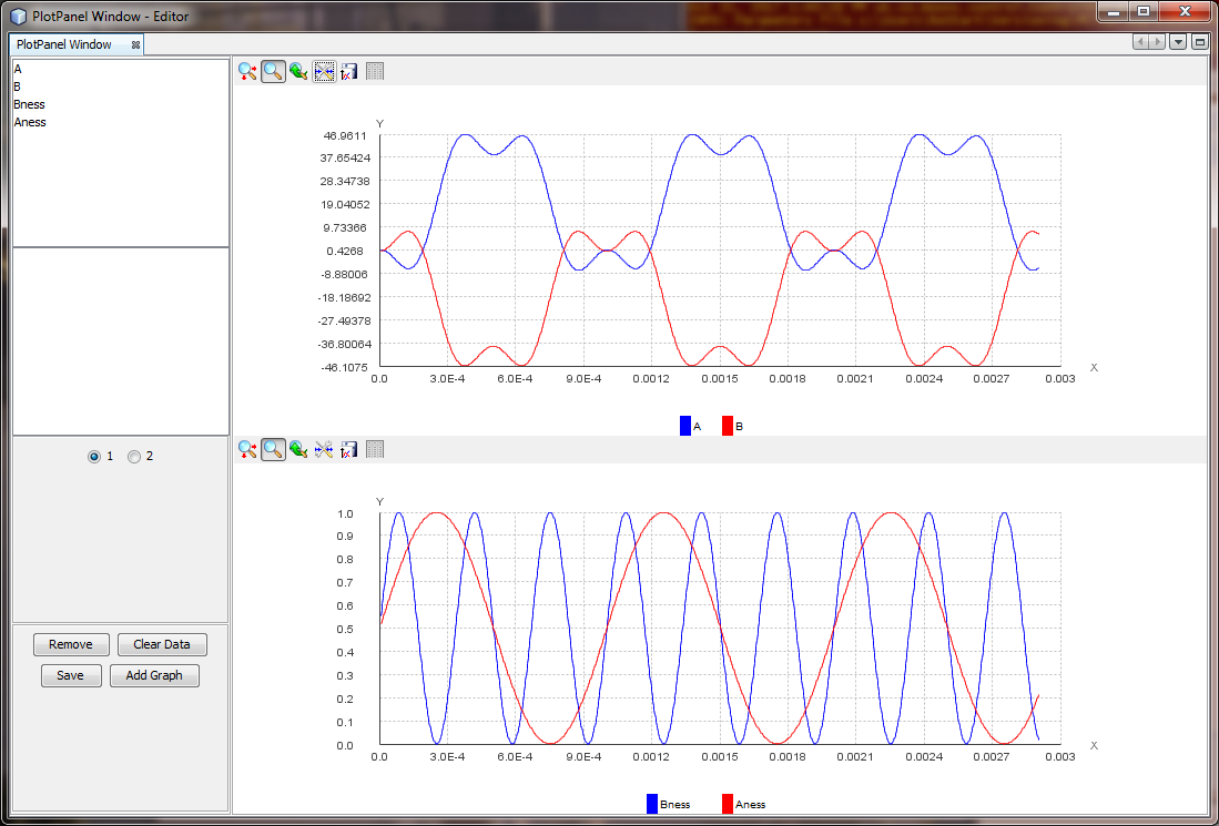
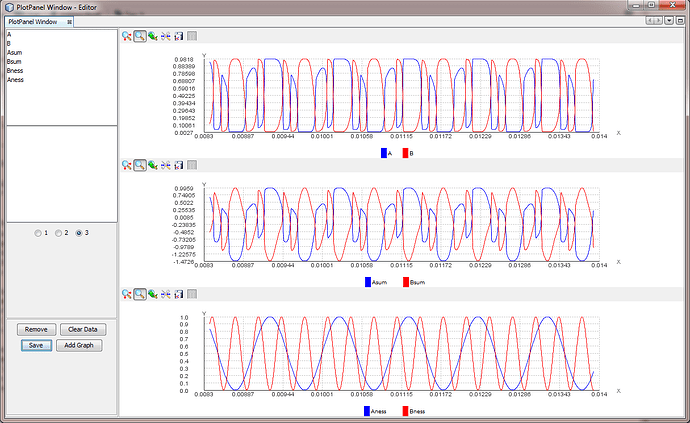
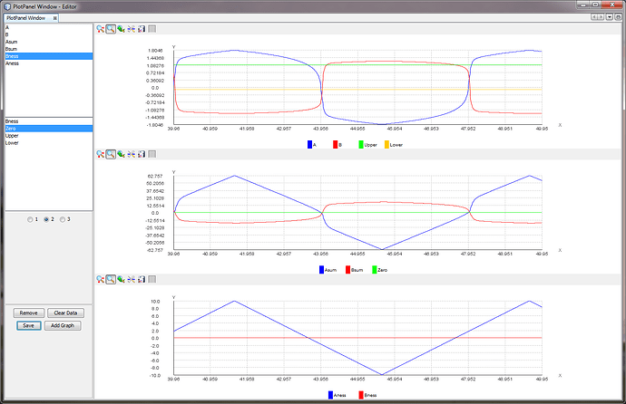
[Martin Taylor 2017.10.29.12.58]
You are right that modelling helps get things correct. Your results
have been puzzling me, so I checked my memory of what I learned so
long ago against Wikipedia’s presentation of flip-flops, with rather
salutary results. I have been mixing two different forms of
flip-flop, analogue and digital and telling you to produce something
that was neither. That’s not helpful. So let’s walk through it
properly, avoiding reliance on my obviously faulty memory.
In the flip-flop described in the Wikipedia article, the equivalent
of PCT perceptual functions are logic circuits that take inputs that
are 1 or 0 and produce outputs that are 1 or 0. It’s binary all the
way. The flip-flop that I argue creates categories is not like that.
It can take as input and produce as output any analogue value
whatever. The flip-flop behaviour whose strength varies from a
slight contrast enhancement to discrete A or B but not both as a
function of some other “modulator” variable (e.g. task stress,
context…) can be represented as a simple cusp catastrophe:

A linear system cannot create such a cusp catastrophe, and I have
been proposing to you a linear system in which the perceptions are
linear functions (sums) of their inputs and the cross-links are
simple multipliers. However, since Weber and Fechner in the mid-19th
century it has been taken for granted that most perceptions are
approximations to logarithmic functions of their inputs rather than
being linear, meaning in our context that the firing rate of a
perceptual output approximates the logarithm of a linear function of
the inputs.
Would changing your "A" and "B" functions to log(Aness + Wba*B) and
log(Bness + WbaA) produce the cusp as the W multipliers decrease
from zero to become increasingly negative? The analysis below
suggests that it might. Obviously, the log cannot be a true
logarithm, because firing rates cannot go below zero, so one would
have to use an approximation to log(X) that does not go below zero
when X <1. Since neither the X-ness nor the A and B outputs can
go below zero, a suitable approximation might be A = log(1+min(0,
Aness+WbaB)). Since Wba*B is the inhibitory influence on the A
perceptual function, its value may be considerably negative, but it
can’t reduce the output below zero, and log(1+X) becomes ever closer
to log(X) as X grows large.
To see whether this nonlinearity will produce the cusp catastrophe,
we could simulate the operation of the circuit or we could analyze.
I trust you to do the simulation, while here I do an informal
analysis. The equations are hard to solve explicitly, so the
analysis is in terms of limits and directions of influence.
Let us look for equilibrium states for A and B, given values of
Aness and Bness, There should be one equilibrium condition if
Wab*Wba is less than a critical value (the analysis below suggests
that this critical value is 1.0) and three if the product exceeds
the critical value. If we make the situation symmetrical by setting
Wab=Wba, we expect one of the equilibrium states to be where A=0,
another where B=0, and a third where A=B. If these turn out to be
equilibrium states, we then have to ask whether they are stable,
metastable, or unstable. If the first two are stable and the third
unstable, all that remains is to determine whether there might be
other equilibria in the dynamic.
If A=0, then Wab*A =0, B=log(1+Bness). Wba*B = Wba*log(1+Bness), the
amount of inhibition of A. Because A = 0, we know that Aness <
-Wbalog(1+Bness). So long as this last inequality holds, A=0,
B=log(1+Bness). We know that this equilibrium is at least
metastable, because it holds for all Aness values less than
-Wbalog(1+Bness). Arguing from symmetry, the other equality B=0, A
= log(1+Aness) is also at least metastable.
But what about A=B? Is that an equilibrium state? It certainly is if
both are zero, which could happen only if Aness and Bness are both
zero. So let’s assume that both are greater than zero, and equal,
because if they are not equal, neither will be A and B.
A = log(1+min(0,Aness+Wba*B)).

By assumption, B=A > 0, so A = log(1+min(0, Aness+Wba*A) =
log(1+Aness+Wba*A) >0
Exponentiating both sides,

e<sup>A</sup> = 1+ Aness +Wba*A

The RHS of this equation grows linearly with A, while the LHS grows
exponentially, …
(Wba=2, Aness = 2)
... and since for A=0 and Aness>0 the LHS is less than the RHS,
there exists for all values of Wba and Aness a value of A for which
the equation holds (LHS=RHS), and the symmetrical expression in B
also holds. So A=B is an equilibrium state. Is it stable? To test
this, we augment Aness by ∂Aness, without changing Bness.
e<sup>A</sup> = 1+ Aness + ∂Aness +Wba*A

To equate the two sides of the equation, e<sup>A</sup> must
increase, meaning that A must increase. What about B? We can no
longer argue from symmetry, so we must examine its corresponding
expression directly.
B = log(1+min(0,Bness+Wab*A). We still know that B >0 (indeed,
before we added ∂Aness, B=A), so we can forget the “min” expression
and exponentiate as before.
e<sup>B</sup> = 1 + Bness + Wab*A

When Aness = Bness, A = B, but now A is greater than it was, so e<sup>B</sup>
is decreased (Wab and Wba are both negative) and so is B. The
reduction in B reduces the inhibition on A, increasing A and further
decreasing B because of the increased inhibition. The A=B
equilibrium is unstable unless Wab = Wba = 0 (the two sides are
unconnected), but there may be a nearby equilibrium value if the
added increase in A is less than ∂Aness, implying a loop gain less
than 1.0.
The loop gain consists of the product of four components, Wab, Wba,
and the derivatives of the perceptual function outputs as a function
of their inputs. Our perceptual functions are “output =
log(1+input)”, for which the derivative is 1/(1+input), so long as
the input is greater than zero. The maximum loop gain occurs where
the total input to a perceptual function (say Aness+WbaB) is just
above zero, where the gain is just under 1.0. The critical point
where the overall loop gain crosses 1.0 therefore occurs when
WabWba ≈ 1. For WabWba >1, there are the three equilibrium
states mentioned earlier, whereas for WabWba<1 there is only
one, near A=Aness, B= Bness for low values of the product,
exaggerating the contrast more and more as the product increases,
until as it increases beyond 1, the steepness of the contrast at A≈B
overlaps and the single equilibrium surface becomes the fold.
 (Modulator
is Wab*Wba in this case, Data is Aness-Bness)
That is an argument from boundary conditions and qualitative
effects. I hope you are able to simulate it and that the simulation
bears out the analysis. If we could have an explicit solution to the
equation eA = 1+ Aness +Wba*A, it would be possible to
provide a proper explicit equilibrium analysis of the loop and have
no doubt.
Sorry for having in my senility led you astray earlier. I hope I'm
not doing that now.
Martin


