For an organism living in an uncertain environment, what matters is
not the state of a perceptual variable, but the state of the
environment. Yet the organism cannot control anything in the
environment; it can control only perceptual variables that are
functions of states of the environment. Ignoring possible inputs
from what in PCT is called “an imagination loop”, the perceptual
input function of a control unit determines a relationship among
properties of the environment that we denote the CEV (complex
environmental variable) of the control unit, the value of which is
denoted “s” in the equations.
The essay begins by considering possible variablility of the CEV
when the perception is controlled but the relation between the CEV
and the perceptual input may have an offset, at first static, and
then variable. This leads to an enquiry into the limits on
perceptual control when there is finite loop delay. Some
experimental tracking runs provide data as a sanity check on the
theoretical limits.
Throughout this essay we consider only a single noise-free control
unit at a single level of control, and assume that the reference
value is static throughout. Consideration of varying reference level
is left for a possible future episode in the series.
Here is a figure with the symbols I use in the equations (plus other
symbols that may be used later).
<img alt="" src="https://mail.google.com/mail/?ui=2&ik=f4dcc9166a&view=att&th=12ceb5d01ecca941&attid=0.1.1&disp=emb&zw" width="272" height="293">
-----------------
Stage 1: static offset (v fixed).
To start, assume a simple static offset of the sensor-perception
alignment, such as happens when a chicken is fitted with prismatic
goggles that make it see everything a little to the right of its
true position. A chicken fitted with such goggles may try to peck at
a seed, but will peck at the earth to the left of the seed. Chickens
seem not to learn to compensate for this offset. If a person is
fitted with such spectacles, the first move to pick up a cup will be
to the left of the handle, but a higher-level control system
controlling perception of the relationship between hand and handle
will change the reference value for the hand movement so that the
hand does eventually meet the handle.
Throughout this essay we consider only a single control unit at a
single level of control, ignoring any possible influences from
higher-level control units, and assume that the reference value is
static throughout.
Here are the control equations, for notational simplicity taking P(
) and E( ) to be the identity transform. The symbols could be simple
variables and operators, or they could be Laplace transforms:
p = P(qi) = qi
= s + v
= (qo + d) + v
= G(e) + d + v
= G(r-p) + d + v
p(1+G) = Gr + d + v
p = Gr/(1+G) + (d+v)/(1+G)
or, in an approximation we use several times hereafter, for G large
p ≈ r + (d+v)/G
In other words, the offset does not affect control of the perception
because the offset simply adds to the influence of the disturbance.
Control still keeps the perceptual value almost the same as its
reference value.
But what of the situation in the environment. What is the value of
the CEV, represented by “s” in the equation? Can the chicken peck
the seed? Does your hand grab the cup handle?
p = qi = s +v, or in other words,
s = p-v ≈ r - v
When the perception is controlled, the CEV has the wrong magnitude;
the chicken does not get to eat the seed, the hand does not meet the
cup handle.
----side note----
If v remains constant, reorganization will probably correct the
problem (though for a human the problem will be resolved by a
changing reference level from a higher level control system that
controls, for example, the relationship between hand and
cup-handle). Indeed, experiments from the 1930s to at least the
1970s showed that under these conditions, when people (but not
chickens) wearing prismatic spectacles act to control some
perception of the outer environment, their perceptual functions
change to compensate for the effect of the prism, but correction
does not happen, or happens much more slowly, for aspects of the
environment observed passively (see work by J.G.Taylor, or by Hein
and Held, and for earlier work the Gestaltists such as Kohler). The
perceptual consequences are sometimes odd, as when an observer who
is wearing spectacles that invert up and down perceives the smoke
from a cigarette to drift downward toward the ceiling above.
----end side note ----
So, a fixed offset between the perceptual signal and the outer world
initially means that actions through the environmental feedback path
result in a feedback effect that mismatches the disturbance value by
the amount of the offset. This displacement probably will be
corrected by reorganization, but for now at least, I want to
consider only the uncorrected raw equations for a single control
system.
-------end Stage 1------------
Stage 2: varying offset (v variable)
The equations are the same as in Stage 1, but now we consider
statistics over some period in which v changes randomly with
Gaussian probability statistics and a mean of zero. Why this might
happen is irrelevant to the argument. Call the offset variance
var(v). We also (for this essay) assume d also varies with Gaussian
statistics, with variance var(d). Since the variations of v and d
are by definition independent, var(d+v) = var(v) + var(d).
The quality of control (Q) is sometimes reported as var(d)/var(p),
or as its square root RMS(d)/RMS(p), which is often called the
“Control Ratio” or CR (sometimes the inverse of those ratios is
used, such as that the RMS variation of the perceptual signal is x%
of the RMS variation of the disturbance). To reduce the number of
symbols in the written form of the equations, I will use Q =
var(d)/var(p), and use CR for its square root when appropriate.
Good control means Q is a large number. if there is no control at
all, Q = 1. If the control system causes the perceptual signal value
to fluctuate more than the disturbance does alone, Q < 1.
As noted above, p ≈ r + (d+v)/G, so if r is constant, var(p) ≈
var(d+v)/G
1/Q ≈ var(p)/var(d)
= (var(d) + var(v)) / (G*var(d))
= (1 + var(v)/var(d)) / G
Q ≈ G/(1 + var(v)/var(d))
The effect of varying v on the quality of control depends on the
relative variances of v and d. If v varies as much as d, the control
is only half as good as it would be if only d varies. (If you use CR
as the measure of control quality, the ratio is sqrt(2)).
That's not very interesting, but what can we say about the effect in
the environment. How does the CEV vary? For example, does the hand
now usually catch the cup handle quite precisely? Does the chicken
usually peck accurately at the seed?
The value of the CEV is denoted by "s" in the equations. For the
hand to catch the cup handle accurately, the mean value of the CEV
should be r (which it is in these equations) and its variance should
be small compared to var(d). Let us have a look.
s = p-v, from the equations of Stage 1.
var(s) = var(p) + var(v) if p and v are uncorrelated, as is nearly
the case when control is good
= ((var(d) + var(v))/G) + var(v)
= var(d)/G + var(v)*(1 + 1/G)
Control reduces the variance component of s due to the disturbance,
but the component due to the varying offset is affected only a small
amount by the fact of control. The variability of s is the variance
of the perceptual offset, plus a little due to the fact that for a
finite gain, control is not perfect. If perceptual control were
perfect, the variance of s would be exactly the variance of the
offset.
That's also not very interesting, since it is intuitively obvious
that if the perceptual value is stable despite having a variable
offset from the value of the CEV, the value of the CEV must be
variable.
This kind of problem cannot be corrected by reorganization, but a
higher-level control system controlling for the relationship between
hand and cup, or between beak and seed, could still function well by
continuously changing the reference value sent to the lower control
system, provided it can act quickly as compared to the rate at which
v varies.
----------end Stage 2-----------
Stage 3. Delay in the loop (v = 0)
The foregoing was just preparation for the core of this essay,
consideration of the effect of loop delay.
In this stage, we forget about the offset v (i.e. we set v = 0
permanently), but let there be loop delay of precisely T seconds.
(For any practically realizable control loop, T would not be a
precise number, but would represent a delay distributed over some
time. But here we consider only the effect of a fixed and precise
delay. Is the effect the same as introducing a variable offset but
no loop delay?
For simplicity in writing the equations, I assume that all the delay
is in the environmental feedback path. It could be anywhere around
the loop for the purposes of the following analysis. I will still
assume that E( ) is a unitary transform, but now it is one with a
delay, such that its input at time t0 appears at its output at time
t1 = t0+T, where T is the loop delay. We start by considering the
situation at time t1.
Now the equations become time-based. Please forgive the notation. I
write p(t1) where I should more properly write p subscript_t1 (t),
but I hope this will nevertheless be intelligible.
p(t1) = s(t1) = d(t1) + qo(t0)
= d(t1) + G(e(t0))
= d(t1) + G(r - p(t0)) (assuming, as before, that r is
static)
Oops! We can't do what we did before, and move Gp across to the left
hand side of the equation to solve for p, because p(t0) differs from
p(t1). We have to continue around the loop, one loop delay at a
time…
p(t1) = d(t1) + G(r - s(t0))
= d(t1) + G(r - (d(t0) + qo(t-1))
= d(t1) + G(r - (d(t0) + G(e(t-1)))
= ....
Round and round the loop we go, creating an infinite equation that
may be possible to evaluate, but not by me.
We no longer have a direct way to compute p(t1) as a function of
d(t1), or even as a joint function of d(t1) and d(t0), because the
influence that opposes the disturbance has a value based on an
earlier value of the disturbance – in fact, on an infinite series
of earlier values. We have to know something about the statistics of
how d varies over time if we are to compute anything exact about
p(t1).
We can, however, determine some limiting conditions.
--------------------------
Stage 4. Limits to control if there is loop delay
Let us assume (against all practical possibility) that qo(t0) would
have been precisely the right value to counter d(t0) exactly if
there had been no loop delay. In other words, if there hadn’t been
any delay, control would have been perfect, giving qo(t0) = r-d(t0).
That’s probably better than the best that can be done by a control
system that does not use any prediction.
The first line in the derivation in Stage 3 above was
p(t1) = s(t1) = d(t1) + qo(t0)
which, using the impractical assumption that qo(t0) = -d(t0),
becomes
p(t1) = s(t1) = dt(t1) - d(t0)
Since the index of the quality of control is
Q = var(d) / var(p)
The interesting question is the distribution of values of p.
If p(t) = d(t) - d(t-T) then
var(p) = var(d(t) - d(t-T)), giving
Q = var(d) / (var(d(t)-d(t-T))
What does the denominator of this expression represent? It is the
variance of the amount by which the disturbance value changes over
the duration of the loop delay, T. If the loop delay is zero, its
value is zero, and Q is infinite (remember we made the assumption
that qo(t0) would have precisely cancelled the effect of the
disturbance, which would mean infinitely good control).
How can we find var(d(t)-d(t-T))?
Assume we know var(d(t)), the overall variance of the disturbance
influence. Assume also that the statistics of the disturbance are
stationary, so that var(d(t-T)) is the same as var(d(t)) for all
delays.
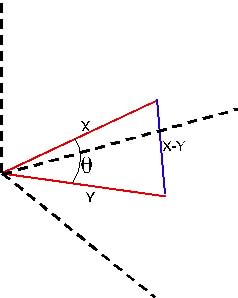
Here we can take advantage of the geometrical interpretation of
correlation http://en.wikipedia.org/wiki/Pearson_product-moment_correlation_coefficient#Geometric_interpretation .
If we have two vectors, X = {x1, x2, …, xn) and Y = (y1, y2, …,
yn), the correlation between the two vectors is the cosine of the
angle between them. Two vectors always define a plane in N-space, as
suggested in the figure.
<img alt="" src="https://mail.google.com/mail/?ui=2&ik=f4dcc9166a&view=att&th=12ceb5d01ecca941&attid=0.1.2&disp=emb&zw" width="238" height="298">
If the two vectors X and Y are taken as two sides of a triangle, the
vector X-Y = {x1-y1, x2-y2, …, xn-yn} is the third side of the
triangle. In the case of interest, X is successive samples of d(t),
Y successive samples of d(t-T), and X-Y is the sample-by-sample
difference d(t)-d(t-T), which is the variable p whose variance we
seek. The lengths of the vectors are the RMS value of the vector
elements, or sqrt(var(vector_elements)). |X| = |Y| = sqrt(var(d)),
X-Y| = sqrt(var(p))
According to the law of cosines, if the sides of a triangle are a,
b, and c, then the length of side c is related to the lengths of the
other two sides and the angle θ between them by the relation
c^2 = a^2 + b^2 - 2ab*cosθ
In our triangle, a is |X|, b is |Y|, and c is|X-Y|.
>X-Y|^2 = |X|^2 + |Y|^2 - 2|X||Y| cosθ
But |X|^2 = |Y|^2 = |X||Y| = var(d),
and cosθ is the correlation between X and Y, which is the
autocorrelation of d(t) at lag = loop_delay, which gives
>X-Y|^2 = var(p) by definition
var(p) = var(d(t) - d(t-T))
= var(d) + var(d) - 2*var(d)(cosθ)
= 2*var(d)(1 - cosθ)
Since X is the disturbance waveform and Y its delayed value, cosθ is
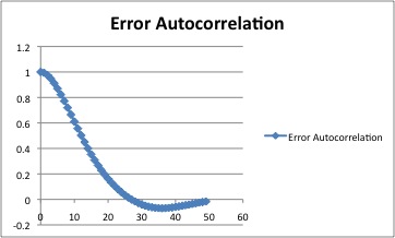
the autocorrelation of the disturbance waveform at lag T. Here’s
what one autocorrelation function selected more or less at random
looks like. The full function is symmetrical about zero lag, and
only half of it is shown. This one happens to be the autocorrelation
function of the error in a real tracking run, but the same sort of
shape is found for many real signals that don’t have sharp spectral
peaks. The abscissa numbers happen to be samples at 60 per second.
<img alt="" src="https://mail.google.com/mail/?ui=2&ik=f4dcc9166a&view=att&th=12ceb5d01ecca941&attid=0.1.3&disp=emb&zw" width="362" height="218">
Finally, from the equations above, we can write the upper bound to
the quality of control for a control loop with loop delay = T.
Qmax = var(d)/(2*var(d)*(1-autocorrel(d at lag T)))
= 1/(2*(1- autocorrel(d at lag T))
No linear control system without prediction can control better than
this (if my assumptions and calculations are reasonable). However,
so long as the disturbance autocorrelation is non-zero at the loop
delay, some prediction is possible, and a control system that does
predict might control better than this formula would suggest.
Whether people predict is a matter for experiment.
The autocorrelation function is the inverse Fourier Transform of the
spectral density function (the spectrum) of the disturbance. So if
you know the spectrum or the autocorrelation function of the
disturbance together with the loop delay of the control system, you
can place an upper bound on the achievable quality of control for a
control system that uses no prediction.
--------Implications--------
If the above analysis is correct, one implication of the result is
that for any lag for which the autocorrelation of the disturbance
waveform is less than 0.5, any attempt to control will be
counterproductive and will result in a perceptual signal that has a
variance greater than that of the disturbance alone. If you think
about it, this makes sense. Consider the extreme case, a loop delay
long enough that the disturbance has zero autocorrelation for that
lag.
To have zero autocorrelation at delay T means that the disturbance
at time t0+T is unrelated to whatever might have happened before
time t0. But any effect of the control system’s output on the CEV
has to have been based entirely on what happened before time t0.
Since s(t) is the sum of the current disturbance and the delayed
output, this means that the variance of the output adds to the
variance of the disturbance rather than reducing it. If qo(t-T)
would have exactly cancelled d(t-T), and d(t) is uncorrelated with
d(t-T), the resulting variance of s is double the variance of d.
What of delays for which the autocorrelation of d is less than 0.5
but greater than zero? One might think that some control would be
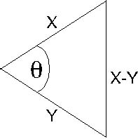
possible. To examine this question, let us go back to the geometric
representation of correlation. Here is the same figure as above, but
drawn flat on the plane. As before, X and Y are proportional to the
square root of the variances of the disturbance and its lagged
version, and cosθ is the correlation between them for some lag. X-Y
represents the sensory variable s if the assumptions above are used.
It is proportional to the square root of the variance of the
sample-by-sample difference between the disturbance and its lagged
version.
<img alt="" src="https://mail.google.com/mail/?ui=2&ik=f4dcc9166a&view=att&th=12ceb5d01ecca941&attid=0.1.4&disp=emb&zw" width="197" height="198">
If cosθ = 0.5, the triangle is equilateral, and the variance of s is
the same as that of the disturbance. In other words, when the
autocorrelation of the disturbance at lag T is 0.5, control is
ineffective at reducing the variability of the perceptual signal,
but is not damaging. For cosθ less than 0.5, the variance of X-Y
exceeds that of the disturbance, and attempts to control would be
counterproductive.
---------Experiment-----------
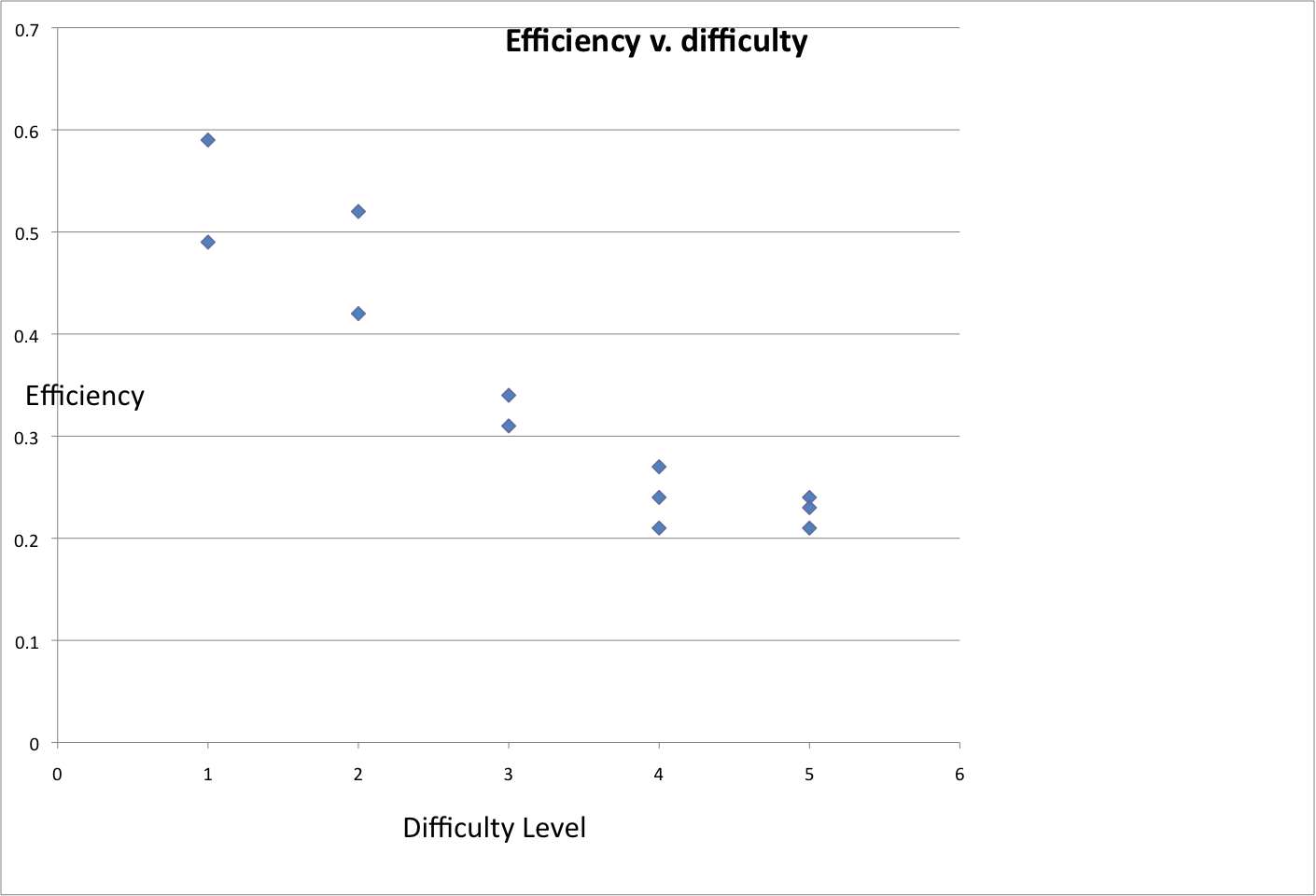
Experimental sanity check of the theory
To test for the sanity of the above analysis, I used Bill P's
“TrackAnalyze” tracking task from LCSIII. I ran 15 tracks using
three different disturbances at each of the five difficulty levels,
and used Excel to determine the disturbance variance and the
perceptual variance, as well as the autocorrelation function of each
disturbance. The autocorrelation values found by plugging the delay
T found by the TrackAnalyze model fit into the data analysis were
mostly in the region of 0.99, far above the “no control” limit of
0.5.
The table shows the results, the left part using variances, the
right part using RMS values. “dif” is the nominal difficulty level
in TrackAnalyze. Q is the ratio of the disturbance variance to the
CEV variance, where the CEV is the target-cursor difference. The
column headed “eff” means “efficiency”, defined to be the actual Q
divided by the maximum possible Q,
Qmax = 1/(2*(1- autocorrel(d at lag T))
from the algorithm above, where T is the model fit loop delay. CR
means the control ratio, the ratio of the RMS values of the
disturbance and the CEV. CR is the square root of the variance ratio
I use in computing Q, and is often used to indicate the quality of
control, since it indicates the ratio of the amplitudes of the
disturbance and the CEV.
The table includes a column headed "L", which will be explained
later.
` dif delay Q Qmax Eff CR CRmax CR/CRmax
L
1 10 36.6 73.8 0.49 6.05 8.59 0.70
12.0
11 32.8 55.2 0.59 5.73 7.43 0.77
12.2
11 32.6 55.2 0.59 5.71 7.43
0.77 10
2 11 14.6 28.4 0.52 3.82 5.33 0.72
10
      10        15.0    35.3    0.42        3.87    5.94    0.65
10.5

      10        15.6    36.5    0.42        3.95    6.04
0.65 10.7
3 9 7.1 23.2 0.31 2.66 4.82
0.55 10.5
      10        5.8     18.1    0.31        2.41    4.25    0.57
10.5

      10        6       17.5    0.34        2.45    4.18
0.59 10.5
4 9 2.7 13.0 0.21 1.64 3.61
0.46 10.6
9 2.9 12.9 0.22 1.70 3.59 0.47
10.5
9 2.8 11.4 0.24 1.67 3.38
0.50 10
5 9 1.47 6.87 0.21 1.21 2.62
0.46 9.2
      9        1.54    6.4     0.24        1.24    2.53    0.49
 10.1

      9        1.58    6.8     0.23        1.26    2.61    0.48
9.3        `
It is encouraging to note that the Q value is reasonably consistent
across runs at the same difficulty level but with different
disturbances, and is always well below the theoretical maximum
possible Q. This provides a sanity check on the theoretical
analysis. A difference of one unit in the loop delay estimate makes
an appreciable difference in Qmax, sufficient to account for all of
the discrepancy in line 1 of difficulties 1 and half the discrepancy
of line 1 of difficulty 2. If the model fit delay in line 1 of
difficulty 3 had been 10 rather than 9, the computed efficiency
would have been about 0.34.
Two trends are apparent in these data. Firstly, the model fitting
suggests that the loop delay is longer for the less difficult tasks.
Even though the same subject (me) did all the tracks (on two
different days), it does make some sense that this should be so.
When the target moves slowly, one is slower to see that a movement
or a change of movement has occurred than when the target moves
quickly.
The other strong trend is that the computed efficiency trends
sharply downward as the difficulty increases. I have not
investigated this, but several possible reasons suggest themselves.
It could signal that the theoretical maximum is too loose, and that
a tighter maximum might be possible to derive. It might be that the
noise inherent in my control actions is relatively more important at
the more difficult levels where control is relatively poor (remember
that the theoretical analysis was based on a completely noise-free
control loop). It could be because the analysis is predicated on a
Gaussian distribution of disturbance values, an assumption that
might be less valid for the more difficult tasks (casual sampling of
the distribution of a few of the disturbance waveforms suggests that
this is not likely to be the problem). It could be because the
analysis assumes a fixed loop transport lag, whereas the transport
lag in the real control system may vary over time. Other reasons may
occur to you.
Variable transport lag seems a viable possibility, since there are
times in the difficult tracks when the target is moving as slowly as
it does most of the time at the easy levels. The noise possibility
also seems plausible and may be worth following up, because the
spectrum of the target-cursor difference waveform (the CEV waveform)
changes across difficulty levels. The following are approximate,
because each CEV waveform is different, and the numbers are by-eye
estimates taken from noisy curves. But the trend is clear for the
CEV waveform to be of higher peak frequency and wider bandwidth as
the difficulty level increases. (Note: these values may be
mis-stated by a factor of 2. I’m not 100% sure of the scale factor
of the Fourier analysis I used).
`Difficulty Spectral peak 6db bandwidth
  1                 0.6 Hx        1.2Hz

  2                 1.2 Hz        1.8Hz

  3                 1.6 Hz        2.0 Hz

  4                 1.6 Hz        2.2 Hz

  5                 2.0 Hz        2.6 Hz   `
I make no interpretation of this trend.
Now I can explain the column "L" in the table. It is the lag in
samples that brings the CEV waveform autocorrelation value to 0.5. I
don’t know whether it is significant that this value is close to the
loop delay estimated by the best fit model, but considering the
importance of autocorrelation = 0.5 in the main analysis, I thought
it worth mentioning in this essay. Further consideration may suggest
that it is a simple coincidence, or perhaps that it has some
rational relationship with the quality of control.
------------------

Further development


All of the above is predicated on a Gaussian distribution of
disturbance values. The reason for this restriction is to permit the
variance analysis. Other distributions require other methods, though
it is often true that using variance analysis gives results that are
not too far wrong. In some future episode I hope to continue this
further.
Martin