Thanks Rick
Now that the discussion has ended by coming full circle, I hope you can tolerate me parking a couple of decidely inexpert observations here.
I share with you (I think) a failure to appreciate why it is so important to Bruce and Luk that other agents are involved in the down-to-earth examples that seem just to be individual control. As well as scenarios A and B, I kept wanting to see a C and even a D option, e.g.
- A - I want to go 60 and can, despite disturbances
- B - I want to go 60 but can’t because of gridlock
- C - I want to go 60 but can’t because a boulder has fallen in the way
- D - I want to go 60 but can’t because the accelerator cable has snapped
Ground zero for all this seems to be the B:CP diagram which Bruce posted, and with which Kent starts his presentation in LCS IV:
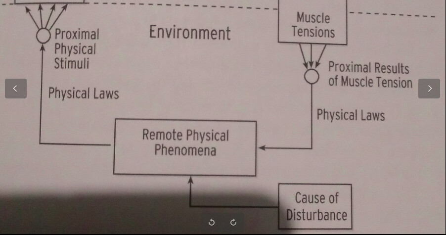
It seems as if other agents and/or collectively maintained resources/substrates with finite capacity have made their way into the “Remote Physical Phenomena” box.
Finally, my inexpert hunch is that disentangling all of this would require scrutinising not just the concept of atenfels (and the ontology of objects as bundles of antenfels?) , but also the relabelling of Remote Physical Phenomena as “CEV”, “Complex Environmental Variable”/“Corresponding Environmental Variable”); and also Martin’s “Mirror World” and importance of Real Reality. These all seem to hang together somehow.
Apologies if this is all terribly wide of the mark - all the best for the conference, I look forward to hearing your reflections on wrongness, Rick! Thanks all for interesting discussion.
Hi John,
Thanks for taking the time to read through the thread. Your scenarios actually highlight the exact structural distinction we are trying to establish, but grouping them all under the umbrella of “I want to go 60 but can’t” masks the underlying mathematics of *why* control is lost. In control theory, that mechanical difference is everything.
Let’s break down your examples:
* **Scenario D (snapped cable):** This is an internal plant failure. The controller’s output ($q_o$) never even reaches the environment. The loop is severed inside your own mechanical boundaries.
* **Scenario C (boulder):** This is a static topological constraint. The physical path simply does not exist.
* **Scenario B (gridlock):** This is **dynamic substrate saturation**. The physical path exists, your car works perfectly, but the local environmental gain ($\partial p / \partial q_o$) has been driven to exactly zero by the active output of *other autonomous agents* ($q_{oB}$ consuming $C_{max}$).
You mentioned sharing a “failure to appreciate” why other agents are so important here, and suggested that shared finite capacity simply makes its way into the “Remote Physical Phenomena” box of the standard B:CP diagram.
That is exactly the crux of the debate. Rick’s position relies on keeping that box permanently closed, treating the environment as a stateless scalar ($k_e$) with an additive disturbance ($d$). Treating Scenario B (gridlock of 5,000 agents) as mathematically identical to Scenario D (a broken gas pedal) completely misses the actual mechanics of the failure.
The mathematical proofs and simulations I provided earlier demonstrate that if you leave that box closed during substrate saturation, the standard math predicts the wrong physical outcome. It fails to account for the structural collapse of the loop and the resulting integrator windup.
The physical environment is not a magic black box with infinite dynamic range. When other agents consume its finite capacity, the loop breaks not from an additive disturbance, but from a physical collapse in environmental gain.
Best,
Luk
1 Like
Yes, that diagram can be misleading. The main problem, for this discussion, is that the feedback path from muscle tension (O) to sensory input (I) goes through “Remote Physical Phenomena” (RPP). The problem is that the actual feedback path in a control loop goes through only a segment of the RPP, the one that forms a causal connection between O and I. For example, the only components of the feedback path in a control loop controlling the speed of your car are the components connecting the accelerator and brake pedals to the spin of the wheels. Other aspects of the RPP, such as passengers in the car, other cars on the road, trees on the hills, etc, are not part of the feedback function in the control of speed loop.
I know that Kent’s diagram is a copy of the one in B:CP so I guess it’s kind of cavelier for me to be criticizing it. But I don’t think Bill ever imagined that anyone would fail to see that the RPP box referred only to remote physical phenomena that are relevant to the control process represented in the diagram.. After all, the RPP box is shown to be in the Environment, which is remote physical phenomena writ large.
I think Bill did a better job of diagramming a control loop in his Science article published the same year as B:CP:
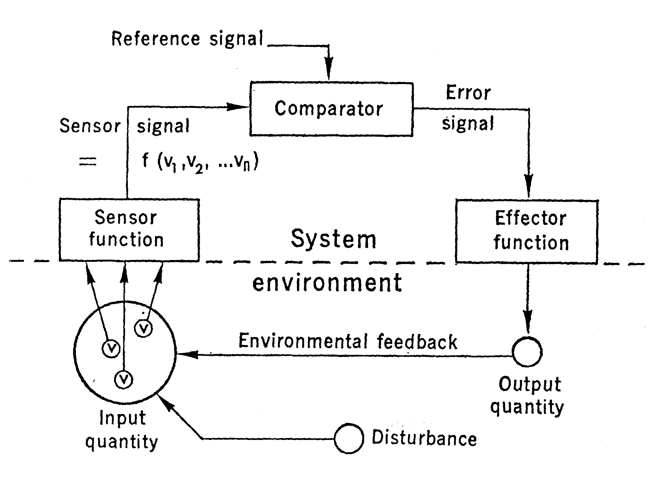
This diagram makes it clear that the “Environmental Feedback” path is the only that part of the environment – AKA remote physical phenomena – that connects O to I. I think it also makes it clearer that the controlled variable – the circled Input Quantity – is a function, f(), of physical variables – the v’s – that can be disturbed by events in the environment (Disturbances) that are independnet of the outputs of the system.
Finally, my inexpert hunch is that disentangling all of this would require scrutinising not just the concept of atenfels (and the ontology of objects as bundles of antenfels?) , but also the relabelling of Remote Physical Phenomena as “CEV”, “Complex Environmental Variable”/“Corresponding Environmental Variable”); and also Martin’s “Mirror World” and importance of Real Reality. These all seem to hang together somehow.
Yes, they hang together in the sense that they are all unnecessary and/or misleading. At least, that’s my experience with them as a modeler. To me, an atenfel is just an ugly name for enities that implement a feedback function, like “motor”, “drive shaft”, “differential”, etc. All you need to know when modeling is the feedback function itself. And CEV is just a misleading name for a CV. Adding the E gives the impression that there is an environmental entity that corresponds to the CV “out there”. But as my “What is Size” demo shows, that’s not quite right. The CV is a function (construction) of the sensory effects of physical variables. So the same physical variables can result in different perceptual variables (such as area and perimeter in the “What is Size” demo) and different physical variables can result in the same perception (as in letter recognition).
The “mirror world” seems to be conflated with the idea that there are entities “out there” in the envirnment , E, called CEVs. These entities don’t exist in PCT. There are just CVs, which are percepual constructions that are functions of E. These are two different models of the perceptual process: the CEV is based on a model of perception as a process of detection (of CEVs), the CV is based on a model of perception as a process of construction (of CVs from E). It is the latter model that is the model of perception used in PCT.
1 Like
Apparently I am not able to communicate my position clearly since what you say above is not my position. But maybe Bill Powers can give you a better sense of how PCT deals with other agents sharing an environment with “finite capacity”. I recommend to you his paper “Degrees of Freedom in Social Interactions” (1979) which is reprinted in “Living Control Systems”. As the title suggests, PCT views other agents as consumers of the finite degrees of freedom in each others’ perceptual worlds rather than as entities that saturate a substrate.
By the way, you can prove a lot of things with math that don’t correspond to what actually happens in the real world. Why not propose some empirical tests of your ideas?
Best, Rick