Ratio control

[Rupert Young 2012.10.27 18.00 BST]

Does anyone have any insight into, or experience with, the control of a
ratio of two values, where one is effected by the output?

The attached shows attempted control (proportional) of two variables, a
"disturbance" and the output. If the disturbance changes the goal of the
control system should be to change the output in order to bring the
ratio back to the reference. As the disturbance rises so should the
output to keep the ratio the same.

In the first sheet of the attached (disturbance is a sine value) control
doesn't seem to work with the normal formulae; even if you try changing
the gain value.

Now, in the second sheet, I have managed to get the control to work by
having a dynamic gain which is a function of the disturbance,
     g = d /(r*r),
that is, the gain is the disturbance divided by the square of the
reference. The third sheet shows a step disturbance.
However, I'm not quite sure why this should work and it doesn't seem
valid, in PCT terms.

Any insight in what is going or here, or the correct way to do it?

ratio-pct.xls (746 KB)

···

--

Regards,
Rupert

[From Bill Powers (2012,10.27.1123 MDT)]

Rupert Young 2012.10.27 18.00 BST --

RY: Does anyone have any insight into, or experience with, the control of a ratio of two values, where one is effected by the output?

The attached shows attempted control (proportional) of two variables, a "disturbance" and the output. If the disturbance changes the goal of the control system should be to change the output in order to bring the ratio back to the reference. As the disturbance rises so should the output to keep the ratio the same.

BP: How about showing the code for the control systems?

I suggest changing the input function so the perceptual signal is the natural logarithm of the controlled quantity:

p = k1*ln(k2*(CV + k3))

This will automatically give you a variation in gain with the amplitude of the CV, and in consideration of Weber-Fechner is something that needs to be investigated. I've always meant to try it but never did. You have to pay attention to the scaling and offset(k2 and k3) so the input to the function never goes negative or to zero, neither of which log functions like.

Best,

Bill P.

···

In the first sheet of the attached (disturbance is a sine value) control doesn't seem to work with the normal formulae; even if you try changing the gain value.

Now, in the second sheet, I have managed to get the control to work by having a dynamic gain which is a function of the disturbance,
    g = d /(r*r),
that is, the gain is the disturbance divided by the square of the reference. The third sheet shows a step disturbance.
However, I'm not quite sure why this should work and it doesn't seem valid, in PCT terms.

Any insight in what is going or here, or the correct way to do it?

--

Regards,
Rupert

[Martin Taylor 2012.10.27.13.12]

I don't see a column in your spreadsheet for the value of the

perceptual signal, which would have to be the ratio that you are
trying to control. I see one input, where I would expect to see the
two that would be needed to create the perception. I haven’t looked
at your formulae, and maybe the second input and the perceptual
signal are hidden there.
Here’s how I would conceive it, assuming both of the variables of
which you want to control the ratio are subject to disturbance, but
only one is influenced by the output (which would presumably be the
usual leaky integrator function).
Is this what is in your spreadsheet formulae?
Martin

···
  [Rupert

Young 2012.10.27 18.00 BST]

  Does anyone have any insight into, or experience with, the control

of a ratio of two values, where one is effected by the output?

  The attached shows attempted control (proportional) of two

variables, a “disturbance” and the output. If the disturbance
changes the goal of the control system should be to change the
output in order to bring the ratio back to the reference. As the
disturbance rises so should the output to keep the ratio the same.

[Martin Taylor 2012.10.27.14.28]

[From Bill Powers (2012,10.27.1123 MDT)]

Rupert Young 2012.10.27 18.00 BST --

RY: Does anyone have any insight into, or experience with, the control of a ratio of two values, where one is effected by the output?

The attached shows attempted control (proportional) of two variables, a "disturbance" and the output. If the disturbance changes the goal of the control system should be to change the output in order to bring the ratio back to the reference. As the disturbance rises so should the output to keep the ratio the same.

BP: How about showing the code for the control systems?

I suggest changing the input function so the perceptual signal is the natural logarithm of the controlled quantity:

p = k1*ln(k2*(CV + k3))

This will automatically give you a variation in gain with the amplitude of the CV, and in consideration of Weber-Fechner is something that needs to be investigated. I've always meant to try it but never did. You have to pay attention to the scaling and offset(k2 and k3) so the input to the function never goes negative or to zero, neither of which log functions like.

For two reasons, would not it be preferable to use (Q = controlled quantity)

p = k*sgn(Q)*ln(abs(Q+offset)) ?

Reason 1: we usually assume that the comparator actually consists of two separate subtractors, one for negative inputs and one for positive, because neurons don't output a negative number of impulses/sec.

Reason 2: the offset has the function of reducing the sensitivity of the logarithm to low-level noise when the signal is near zero. (equivalent to a tolerance zone).

Martin

[From Bill Powers (2012.28.0930 MDT)]

Martin Taylor 2012.10.27.14.28 --

For two reasons, would not it be preferable to use (Q = controlled quantity)

p = k*sgn(Q)*ln(abs(Q+offset)) ?

Reason 1: we usually assume that the comparator actually consists of two separate subtractors, one for negative inputs and one for positive, because neurons don't output a negative number of impulses/sec.

Reason 2: the offset has the function of reducing the sensitivity of the logarithm to low-level noise when the signal is near zero. (equivalent to a tolerance zone).

BP: Both are excellent ideas. Obviously a pure log function doesn't handle small quantities correctly to serve as neural models -- for inputs decreasing from 1 to 0, the output is a rapidly growing negative number!. And your point about positive and negative errors requiring two comparators is important because the real neurons have to work that way no matter what function we use to represent them. The signum (sgn) function effectively provides the separate treatments.

Best,

Bill P.

ratio-pct v1.0.xls (289 KB)

···

[From Rupert Young 2012.10.28 18.00 UT]

  Bill Powers (2012.28.0930 MDT)

  Martin Taylor 2012.10.27.14.28 --

  Thanks. Responding to both.

  MT: p = k*sgn(Q)*ln(abs(Q+offset))   ?

  BP: Both are excellent ideas....

  Following perceived consensus I've used the above formula. To

confirm if I am applying correctly, in the attached I have,

  •       output(t) - the starting output value (o), which is also an
    

    input to the controlled variable

  • sine - a sine varying value, which varies from 0 to 1

  •       input - (i) which is one of the inputs to the controlled
    

    variable, the ratio, in this instance input is the same as the
    sine varying value

  •       ratio - the ratio of two variables, the input and output,
    

    and = i/o. This is the controlled variable, Q.

  •       perc - the value of the perceptual signal (p) using the
    

    above formula

  •       ref - the reference value (r). If it is 0.01 then when the
    

    value of i =1.0 the value of o should = 100.

  • err - the error signal (e), e = r - p

  •       gain - a static gain value (g), if negative it ensures the
    

    output is positive

  •       output(t+1) - the output value at the end of each iteration
    

    and is computed with a proportional integrator function,
    o(t+1) = o(t)+g*e

  • the values of k and offset are in cells L2 and L3

    As can be seen in the spreadsheet the shape of the perceptual
    

signal is the same as the ratio and control is not working, so I
must be doing something wrong. Any suggestions?

  On 28/10/2012 15:36, Bill Powers wrote:
Regards,
Rupert
  [From Bill Powers (2012.28.0930 MDT)]


  Martin Taylor 2012.10.27.14.28 --
    For two reasons, would not it be

preferable to use (Q = controlled quantity)

    p = k*sgn(Q)*ln(abs(Q+offset))   ?


    Reason 1: we usually assume that the comparator actually

consists of two separate subtractors, one for negative inputs
and one for positive, because neurons don’t output a negative
number of impulses/sec.

    Reason 2: the offset has the function of reducing the

sensitivity of the logarithm to low-level noise when the signal
is near zero. (equivalent to a tolerance zone).

  BP: Both are excellent ideas. Obviously a pure log function

doesn’t handle small quantities correctly to serve as neural
models – for inputs decreasing from 1 to 0, the output is a
rapidly growing negative number!. And your point about positive
and negative errors requiring two comparators is important because
the real neurons have to work that way no matter what function we
use to represent them. The signum (sgn) function effectively
provides the separate treatments.

  Best,


  Bill P.

Hi Bill,

Bill P :
And your point about positive and negative errors
requiring two comparators is important because the real neurons have
to work that way no matter what function we use to represent them.

HB :
Can you elaborate this statement simultanously with physiological and PCT explanations ?
Neuron seems to me like physiological term.

Best,

Boris

···

----- Original Message ----- From: "Bill Powers" <powers_w@FRONTIER.NET>
To: <CSGNET@LISTSERV.ILLINOIS.EDU>
Sent: Sunday, October 28, 2012 4:36 PM
Subject: Re: Ratio control

[From Bill Powers (2012.28.0930 MDT)]

Martin Taylor 2012.10.27.14.28 --

For two reasons, would not it be preferable to use (Q = controlled quantity)

p = k*sgn(Q)*ln(abs(Q+offset)) ?

Reason 1: we usually assume that the comparator actually consists of two separate subtractors, one for negative inputs and one for positive, because neurons don't output a negative number of impulses/sec.

Reason 2: the offset has the function of reducing the sensitivity of the logarithm to low-level noise when the signal is near zero. (equivalent to a tolerance zone).

BP: Both are excellent ideas. Obviously a pure log function doesn't handle small quantities correctly to serve as neural models -- for inputs decreasing from 1 to 0, the output is a rapidly growing negative number!. And your point about positive and negative errors requiring two comparators is important because the real neurons have to work that way no matter what function we use to represent them. The signum (sgn) function effectively provides the separate treatments.

Best,

Bill P.

[From Bill Powers (2012.10.30.0815 MDT)]

Bill P :
And your point about positive and negative errors
requiring two comparators is important because the real neurons have
to work that way no matter what function we use to represent them.

HB :
Can you elaborate this statement simultanously with physiological and PCT explanations ?
Neuron seems to me like physiological term.

It is. A comparator can be constructed with a neuron that receives an excitatory reference signal and an inhibitory perceptual signal. The magnitude of the error signal will then be the amount by which the excitation exceeds the inhibition.

However, if the excitation is less than the inhibition, there will never be any error signal output. It's not possible for one neuron to compute both positive and negative error signals. Therefore if a control system does handle both positive and negative errors, there must be two comparators, one as just described and a second one with the perceptual signal being excitatory and the reference signal being inhibitory.

Another way to arrive at the same conclusion is to recognize that neural signals are measured in impulses per second. Again, it's not possible for one neural signal to represent both positive and negative values of the same variable. The firing rate can represent one sign of the variable but not both, since firing rates can't go negative.

Best,

Bill P.

···

At 02:53 PM 10/30/2012 +0100, boris_upc wrote:

Hi,

BP :

A comparator can be constructed with a neuron that receives an

excitatory reference signal and an inhibitory perceptual signal. The
magnitude of the error signal will then be the amount by which the
excitation exceeds the inhibition.

However, if the excitation is less than the inhibition, there will never
be any error signal output. It's not possible for one neuron to compute
both positive and negative error signals. Therefore if a control system
does handle both positive and negative errors, there must be two
comparators, one as just described and a second one with the perceptual
signal being excitatory and the reference signal being inhibitory.

HB :

How do you suppose the hierarchical behavioral control structure in PCT works ?

For example the figure on page 191 in B:CP, 2005.

What kind of neurons or comparators build behavioral hierarchy ?

Inhibitory reference, excitatory reference, mixed ?

How do neuron knows which signal is reference in both cases ?

Best,

Boris

···

----- Original Message ----- From: "Bill Powers" <powers_w@FRONTIER.NET>
To: <CSGNET@LISTSERV.ILLINOIS.EDU>
Sent: Tuesday, October 30, 2012 3:25 PM
Subject: Re: Ratio control

[From Bill Powers (2012.10.30.0815 MDT)]
At 02:53 PM 10/30/2012 +0100, boris_upc wrote:

Bill P :
And your point about positive and negative errors
requiring two comparators is important because the real neurons have
to work that way no matter what function we use to represent them.

HB :
Can you elaborate this statement simultanously with physiological and PCT
explanations ?
Neuron seems to me like physiological term.

It is. A comparator can be constructed with a neuron that receives an
excitatory reference signal and an inhibitory perceptual signal. The
magnitude of the error signal will then be the amount by which the
excitation exceeds the inhibition.

However, if the excitation is less than the inhibition, there will never
be any error signal output. It's not possible for one neuron to compute
both positive and negative error signals. Therefore if a control system
does handle both positive and negative errors, there must be two
comparators, one as just described and a second one with the perceptual
signal being excitatory and the reference signal being inhibitory.

Another way to arrive at the same conclusion is to recognize that neural
signals are measured in impulses per second. Again, it's not possible for
one neural signal to represent both positive and negative values of the
same variable. The firing rate can represent one sign of the variable but
not both, since firing rates can't go negative.

Best,

Bill P.

[From Bill Powers (2012.10.21.1620 MDT)]

Rupert Young 2012.10.28 18.00 UT]

Bill Powers (2012.28.0930
MDT)

MT: p = k*sgn(Q)*ln(abs(Q+offset)) ?

BP: Both are excellent ideas…

Following perceived consensus I’ve used the above formula. To confirm if
I am applying correctly, in the attached I have,

  • output(t) - the starting output value (o), which is also an input to
    the controlled variable
  • sine - a sine varying value, which varies from 0 to 1
  • input - (i) which is one of the inputs to the controlled variable,
    the ratio, in this instance input is the same as the sine varying value
    BP: Let’s back off and start out simpler. The log function is the
    key here. Instead of looking at ratios right away, let’s just look at an
    ordinary control system that happens to have a log function as a
    perceptual input function. That’s Martin Taylor’s suggested
    form:

MT: p =
k*sgn(Q)*ln(abs(Q+offset)) ?

The reference signal has to be in the same units as the perceptual
signal. In order to get a comparison and an error signal we use the same
form of comparator as always:

e = r - p;

But what does this mean in terms of the natural log function ln(x)? I’ll
leave out the scaling and offset values to keep the equations from
getting cluttered. The correspondence of the externally observed value of
the controlled quantity cv to the perceptual signal is, first forward
then backward,

p = ln(cv) or cv = exp(p).

For the reference signal, it is

r = ln(cv’) or cv’ = exp(r)

where the prime (') indicates the reference value.

From this we can get the correspondence of zero error to the actual and
desired states of the controlled variable:

e = r - p = ln(cv’) - ln(cv)

Note that the difference in magnitude between r and p is ln(cv’) -
ln(cv), which is the same thing as ln(cv’/cv), the log of the ratio of
the desired to actual values of the controlled variable. So now the error
signal, instead of representing the difference between desired and actual
values of the cv, represents the ratio of desired to actual values. When
p = r, the error signal is zero as usual, but now that means that the
ratio of cv’ to cv is now 1.0. The natural log of 1 is zero.

cv’/cv = 1.0

But – how handy! – this means that cv’ = cv. which of course is what we
want. When p = r, the actual value of the cv is equal to the desired
value cv’ that we can determine by using the TCV. So we get the same
values of cv and cv’ from The Test that we would get in the linear case.
In fact we can’t even see that a log function is interposed.

The difference is in what an error signal means, and for small errors
there is very little difference. For larger errors, an error signal of
(for example) +2.0 units now does not mean that p is less than r by 2.0
units; it means that the ratio, cv’/cv is exp(2.0), so the desired value
of the cv is 7.39 times the actual value, or the actual cv is 0.135 of
the desired cv. If the error is 10.0 units, the cv is 0.0000454 of cv’.
An infinite positive error means the perceptual signal is zero. Of course
for such large errors we would not expect the perceptual input function
to follow the ideal logarithmic curve over its whole range.

I leave it to the reader to put the offsets and scaling factors back into
the equations and see how all this comes out – I have to go tend to my
front door and ghosts and goblins slavering for candy. This will count
for 1/pi of your grade. When you translate the results into the behavior
of the CV and the behavioral output, you should get familiar
results.

Concerning the output, the easiest way to start is just to let the output
be the integral of the error signal. The pure integral is a good place to
start; you can then experiment with the effects of using a leaky
integral. With a pure integral the system should be stable over a wide
range of error signals; with a leaky integral, not so wide.

Good luck.

Best,

Bill P.

[Rupert Young 2012.11.01 22.00 UT]

From Bill Powers (2012.10.21.1620 MDT)

BP: Let's back off and start out simpler. The log function is the key here....

RY: Thanks that's beginning to make more sense to me. I'm away for a few days and will have a look in more detail next week.

Regards,
Rupert

[Rupert Young 2012.11.05 19.00 UT]

ratio-pct v1.3.xls (647 KB)

···

From Bill Powers (2012.10.21.1620 MDT)

          BP: Let's back off and start out simpler. ... The

reference signal has to be in the same units as the
perceptual signal.

      RY: Ok, I now have, in the attached, both the reference and

perceptual signals in equivalent terms, using the natural
logarithm.

The reference signal r=k*sgn(ref)*ln(abs(ref+off)),

where ref is the desired ratio of the two input values.

ratio = b/a,

where “b” is a disturbance and “a” is the output.

          BT: I leave it to the reader to put the offsets and

scaling factors back into the equations and see how all
this comes out

      RY: I have tried different values for these. For the offset

changing this to >= 1 avoids negative values. I’m not sure
the use of the scaling factor, though it seems to correspond
to the slowing factor in the leaky integrator.

          BT: Concerning the output, the easiest way to start is

just to let the output be the integral of the error
signal. The pure integral is a good place to start; you
can then experiment with the effects of using a leaky
integral.

      RY: I have used the leaky integrator, I think, o = o + s

(g*e-o), what is the pure integrator?

      Further than this I am still struggling with my model.

Using a step function (see sheet LN Perc Step) for “b” control
is successful once “b” becomes constant.

      However, using a sine function (see sheet LN Perc Sine) for

“b” control doesn’t appear to work. The values of the sine
function are between 0 and 1. With a ratio reference of 0.001
the output should come to 1000. I have tried changing the
values of slow and gain, but can’t get seem to get this to
work. Or maybe control is successful but is lagging behind the
sine function. Perhaps there is a flaw in using values between
0 and 1 for “b”.

Any idea what I am doing wrong?

Regards,

Rupert

[From Bill Powers (2012.11.05.1355 MST)]

Rupert Young 2012.11.05 19.00 UT

More on this later.

RY: I have used the leaky
integrator, I think, o = o + s (g*e-o), what is the pure
integrator?

It’s just o = o + gedt.

There should be a dt in the leaky integrator version, too, defining the
length of time represented by one iteration of the program.

However, using a sine function
(see sheet LN Perc Sine) for “b” control doesn’t appear to
work. The values of the sine function are between 0 and 1. With a ratio
reference of 0.001 the output should come to 1000. I have tried changing
the values of slow and gain, but can’t get seem to get this to work. Or
maybe control is successful but is lagging behind the sine function.
Perhaps there is a flaw in using values between 0 and 1 for
“b”.

The trick here is to look at the behavior of each variable and see if it
makes sense. First, set the two inputs to values with a ratio somewhere
near 1 (say, between 0.1 and 10.0) and see what the perceptual signal is.
Vary one of the inputs and see how the perceptual signal changes. This
will show you the range of values of the perceptual signal. Set the
reference signal somewhere within this range, and look at the error
signal. Then close the loop and with the disturbing variable constant,
see how the output changes the other input variable and whether that
variable approaches the correct value. You can adjust dt to make the
approach to the final values happen in a reasonable time – not too fast,
not too slow. You may find at this stage that a gain is much too large,
or much too small. You may find that a sign is wrong so the error gets
larger instead of smaller as each dt goes by.
To make sense of this system you must understand how each part of it
works
, not just enter equations and run the program. Put the final
model together piece by piece and don’t move on to the next piece until
you understand the previous pieces. By “understand” I mean to
figure out what you should see, then check to see if that is what
happens. If the inputs are a = 10 and b = 20, then what should the
perceptual signal be? Is that what it is? Then subtract the perception
from the reference and see what the error is. Then after one iteration
check the error again and see if it’s changing the right way and by a
reasonable amount. And so on.

The first time you do this it can get pretty tedious, but you will
quickly get better at it. You’ll soon be able to do most of it in your
head without even running the program.

If you figure out for yourself what is wrong, you will never forget it.
If I figure it out and tell you, you will just memorize an action, which
will probably be the wrong one next time.

Best,

Bill P.

ratio-pct v1.4.xls (780 KB)

···

[From Rupert Young 2012.11.06 23.30 UT]

  Bill Powers (2012.11.05.1355 MST)

  BT: If you figure out for yourself what is wrong, you will never

forget it.
If I figure it out and tell you, you will just memorize an action,
which
will probably be the wrong one next time.

  RY: That makes sense, and I appreciate your guidance on this

matter; though you may be overestimating my ability to work it
out! Btw, are you aware of what is wrong, or are you just
suggesting approaches for investigation?

  BT: To make sense of this system you must *        understand how each

part of it
works* , not just enter equations and run the program. Put the
final
model together piece by piece and don’t move on to the next piece
until
you understand the previous pieces.

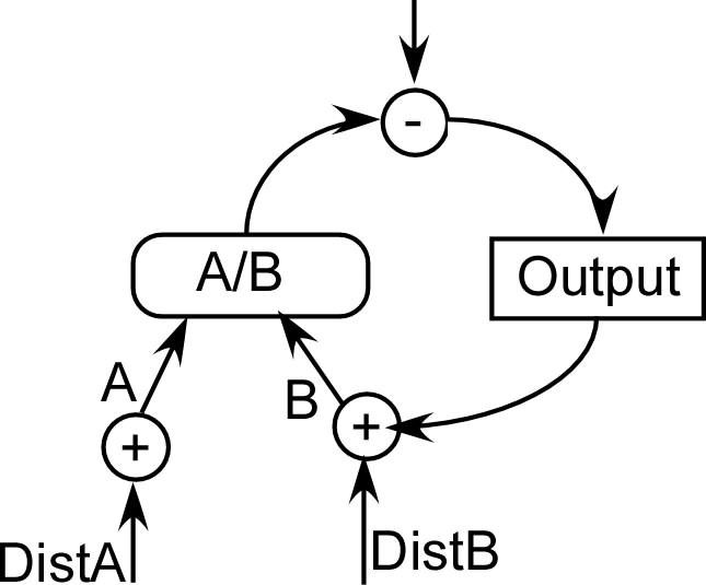
  RY: I was trying to do something like that (the third and fourth

sheets of the spreadsheet had a control system using a constant
disturbance and a plot of ln values), but kept getting stuck.
However, I’ve had another go along the lines you suggested, using
the third sheet (ln int) in the attached.

  If a = b = 3 then ratio = 1 and ln(ratio) = 0

  If a = 3 and b = 9 then ratio = 3 and ln(ratio) = 1.099

  If a = 3 and b = 27 then ratio = 9 and ln(ratio) = 2.197

  If a = 3 and b = 81 then ratio = 27 and ln(ratio) = 3.296

  I note that as the ratio increases by a multiple of 3 then the

ln(ratio) increases by 1.099, which is also ln(3).

  Closing the loop and using a pure integral and starting with a = b

= 3,

  if reference is 0.1 the output slowly approaches the target of 30,

  as the reference increases from 0.1 to 10 the output approaches

its target more quickly,

  around 12 the output oscillates around the target,

  13 and higher and the system becomes out of control

  So here I run into an impasse again, as normally, with a

“standard” control system, increasing the reference would just
result in a longer time for the system to become under control
(wouldn’t it?).

  Though row 4 (highlighted in sheet "ln int") doesn't look right.

The starting output is 0.714 and the target, that would bring the
ratio to the reference 13, is 0.23, with a gain of -0.5 one would
expect that g*e would represent half the amount between 0.714 and
0.23, but in this case it is 0.565, which means it overshoots. So
is it the case then that the error, and, therefore, the change
that we are applying to the output is not in the right units?

  It's late, so I'll sleep on it; though any hints welcome.

  Regards,

  Rupert

  On 05/11/2012 21:37, Bill Powers wrote:

[From Bill Powers (2012.11.05.1355 MST)]

  Rupert Young 2012.11.05 19.00 UT


  More on this later.
    RY: I have used the

leaky
integrator, I think, o = o + s (g*e-o), what is the pure
integrator?

  It's just o = o + g*e*dt.


  There should be a dt in the leaky integrator version, too,

defining the
length of time represented by one iteration of the program.

    However, using a sine

function
(see sheet LN Perc Sine) for “b” control doesn’t appear to
work. The values of the sine function are between 0 and 1. With
a ratio
reference of 0.001 the output should come to 1000. I have tried
changing
the values of slow and gain, but can’t get seem to get this to
work. Or
maybe control is successful but is lagging behind the sine
function.
Perhaps there is a flaw in using values between 0 and 1 for
“b”.

  The trick here is to look at the behavior of each variable and see

if it
makes sense. First, set the two inputs to values with a ratio
somewhere
near 1 (say, between 0.1 and 10.0) and see what the perceptual
signal is.
Vary one of the inputs and see how the perceptual signal changes.
This
will show you the range of values of the perceptual signal. Set
the
reference signal somewhere within this range, and look at the
error
signal. Then close the loop and with the disturbing variable
constant,
see how the output changes the other input variable and whether
that
variable approaches the correct value. You can adjust dt to make
the
approach to the final values happen in a reasonable time – not
too fast,
not too slow. You may find at this stage that a gain is much too
large,
or much too small. You may find that a sign is wrong so the error
gets
larger instead of smaller as each dt goes by.

  To make sense of this system you must *        understand how each part

of it
works* , not just enter equations and run the program. Put the
final
model together piece by piece and don’t move on to the next piece
until
you understand the previous pieces. By “understand” I mean to
figure out what you should see, then check to see if that is what
happens. If the inputs are a = 10 and b = 20, then what should the
perceptual signal be? Is that what it is? Then subtract the
perception
from the reference and see what the error is. Then after one
iteration
check the error again and see if it’s changing the right way and
by a
reasonable amount. And so on.

  The first time you do this it can get pretty tedious, but you will

quickly get better at it. You’ll soon be able to do most of it in
your
head without even running the program.

  If you figure out for yourself what is wrong, you will never

forget it.
If I figure it out and tell you, you will just memorize an action,
which
will probably be the wrong one next time.

  Best,


  Bill P.

[From Bill Powers (2012.11.07.0625 MST)]

Rupert Young 2012.11.06 23.30 UT --

BP earlier: If you figure out for yourself what is wrong, you will never forget it. If I figure it out and tell you, you will just memorize an action, which will probably be the wrong one next time.

RY: That makes sense, and I appreciate your guidance on this matter; though you may be overestimating my ability to work it out! Btw, are you aware of what is wrong, or are you just suggesting approaches for investigation?

BP: No, I haven't tried to figure it out. I expect you to save me the trouble.

RY: If a = b = 3 then ratio = 1 and ln(ratio) = 0
If a = 3 and b = 9 then ratio = 3 and ln(ratio) = 1.099
If a = 3 and b = 27 then ratio = 9 and ln(ratio) = 2.197
If a = 3 and b = 81 then ratio = 27 and ln(ratio) = 3.296

I note that as the ratio increases by a multiple of 3 then the ln(ratio) increases by 1.099, which is also ln(3).

Closing the loop and using a pure integral and starting with a = b = 3,

if reference is 0.1 the output slowly approaches the target of 30,
as the reference increases from 0.1 to 10 the output approaches its target more quickly, around 12 the output oscillates around the target, 13 and higher and the system becomes out of control

So here I run into an impasse again, as normally, with a "standard" control system, increasing the reference would just result in a longer time for the system to become under control (wouldn't it?).

BP: Yes, but only if the system remains stable. In the logarithmic model, increasing the value of a variable also increases the gain, because the slope of the curves changes. Even in the linear case, increasing the gain too much can cause instability.

Try reducing the value of dt. If the steps between iterations become too large, the linear approximation is not accurate enough and the system can become "computationally unstable," meaning that the instability is just a matter of an inaccurate simulation. There are methods of integration such as "Runge-Kutta" which do allow larger steps and thus fewer computations, but it's usually simpler just to make the time-steps smaller.

This is good progress. Reduce dt and see what happens. By the way, how about including the program steps for the control system, or just the equations? I'nm too lazy to try to find them in previous posts.

RY: Though row 4 (highlighted in sheet "ln int") doesn't look right. The starting output is 0.714 and the target, that would bring the ratio to the reference 13, is 0.23, with a gain of -0.5 one would expect that g*e would represent half the amount between 0.714 and 0.23, but in this case it is 0.565, which means it overshoots. So is it the case then that the error, and, therefore, the change that we are applying to the output is not in the right units?

BP: No, it's that the program assumes a linear change whereas the functions involved are nonlinear because of the log function. The smaller dt is, the less difference there is between a short linear extrapolation and the true logarithmic one. With a smaller dt, more computations are needed to cover a given time span, but the accuracy increases. I'm sure your computer is fast enough that you could make dt a lot smaller, especially if you're not using an explicit value of dt, which makes dt = 1. Try making it 0.01.

Best,

Bill P.

[From Rupert Young 2012.11.07 23.30 UT]

(Bill Powers (2012.11.07.0625 MST)

BP: By the way, how about including the program steps for the control system, or just the equations? I'nm too lazy to try to find them in previous posts.

RY: It's in a spreadsheet. There are two variables, "a", which is affected by the output (in this case it is the output) and "b", a disturbance.

The ratio rt = b/a.

The perceptual signal p = k . sgn(rt) . ln(abs(rt +off), where k is a scaling factor and off is an offset.

If the reference, representing a target ratio of two variables, is r' then the reference signal, used in the comparator, is r = k . sgn(r') . ln(abs(r' +off).

The error signal e = r - p.

The output is o(i+1) = o(i) + g . e, where "i" indicates the iteration. And o(i+1) becomes variable "a" in the next iteration.

BP: Try reducing the value of dt.

RY: Do you mean reduce the sampling rate? In my current model there is no explicit value of dt, as it is a spreadsheet and each row represents the change in time, and I don't have a variable that is sampled (the disturbance is constant). Or am I misunderstanding?

Regards,
Rupert

[From Bill Powers (2012.11.07.2040 MST)]

Rupert Young 2012.11.07 23.30 UT --

BP earlier: Try reducing the value of dt.

RY: Do you mean reduce the sampling rate? In my current model there is no explicit value of dt, as it is a spreadsheet and each row represents the change in time, and I don't have a variable that is sampled (the disturbance is constant). Or am I misunderstanding?

I mean put an explicit dt into every integration and then reduce its size, so the change in the integral during any one iteration is smaller. You need some way to tie one iteration to the elapsed time represented by one iteration, anywhere there is a function of time. One iteration can represent one second, or 0.001 second. The amount by which an integral changes in one second is much greater than than the amount it would change in one millisecond. When you plot the results, the time axis will appear much more stretched out when each pixel in the x direction represents one millisecond. You still do one iteration of the spreadsheet at a time, but the physical time along the x axis is different when you change dt.

Best,

Bill P.

[From Rupert Young 2012.11.09 21.30 UT]

Bill Powers (2012.11.07.2040 MST)

BP: I mean put an explicit dt into every integration ...

RY: Gotcha, I'll give it a go.

With regards to the ratio control I think I've actually made some real
progress.

In the attached you can see control works well for a large range of
values, with a constant disturbance (sheet "ln int o.g.e"). Also with a
sine disturbance, values between 0 and 1 (sheet "LN Perc Sine - Pure"),
though there is high error when the disturbance is close to zero, but
this is because there are large proportional differences, with the
disturbance, between iterations.

After examining how the variables behaved I came to the conclusion that
there was a problem with how the output was computed.

Normally the input to the perceptual function would be of the form,

i = o + d, where o is the output from a previous iteration, and d is a
disturbance. The function is a sum and all components contribute in an
additive way.

If output is of the form o' = o + g.e, then

i = o + g.e + d.

That is, the change (g.e) to the output is also an additive adjustment
to the input.

However, in terms of ratio control,

i = d / o, and if we were to stick with the same output function,

i = d / (o + g.e).

However, this doesn't seem right as the change (g.e) is still acting as
an additive element whereas it should be contributing to the input as a
denominator.

So, can we express the change in such a way that it will act as a
denominator?

Well, if we think of the input as

i = d / f(o), that is we are dividing d by o and any changes to o we can
achieve that by multiplying the the change element within this equation
by 1/o, which means the change would be o.g.e, that is the output
function would be,

o' = o + o.g.e.

This seems to work though I am not sure my reasoning is quite right.
Maybe you can express it better than I, verbally and mathematically.

Regards,
Rupert

ratio-pct v1.6.xls (1.22 MB)

[From Bill Powers (2012.11.17.1102 MST)]

Rupert Young 2012.11.09 21.30 UT --

RY: After examining how the variables behaved I came to the conclusion that there was a problem with how the output was computed.

Normally the input to the perceptual function would be of the form,

i = o + d, where o is the output from a previous iteration, and d is a disturbance. The function is a sum and all components contribute in an additive way.

If output is of the form o' = o + g.e, then

i = o + g.e + d.

This should be

i = o'+ d

because o' is the value of the output after the current iteration. To make this clearer, you could include a time index for e, o and i (I use * for multiplicaton):

o[t] = o[t-1] + g*e[t-1]*dt /new output = old value plus (gain * old error * dt)

i[t] := o[t] + d[t] / new input quantity = current output + current disturbance

There is no reason to convert into the equivalent log terms because there are no log functions in the environment of this system. Only the perceptual input function receives a scalar input and produces an output that is a log function of that input.

If there were also a logarithmic perceptual input function receiving information about the magnitude of the disturbance, the output of that function would be the log of the disturbance magnitude. A second-order input function computing the sum of the log input quantity and the log disturbance would then represent log(d*i). But the disturbance is not represented as a perception in this model; only the input quantity is represented.

Sorry for the delay...

Best,

Bill P.

[From Rupert Young 2012.11.20 22.00 UT ]

Bill Powers (2012.11.17.1102 MST)

RY: i = o + g.e + d.

BP: This should be i = o'+ d

RY: I probably wasn't expressing myself very well.

Using your terminology:

(1) o[t] = o[t-1] + g*e[t-1]*dt /new output = old value plus (gain * old error * dt)

(2) i[t] := o[t] + d[t] / new input quantity = current output + current disturbance

If we substitute o[t] in (2) with the right-hand side of (1) we get,

i[t] := o[t-1] + g*e[t-1]*dt + d[t].

Yes? That is, the input to a new iteration is a function of the previous output and a linear additive adjustment (g*e[t-1]*dt), and the disturbance.

In ratio control, however,

(3) i[t] := d[t] / o[t] / new input quantity = current disturbance / current output

and I am questioning whether equation (1) is valid in this situation, which would give

(4) i[t] := d[t] / (o[t-1] + g*e[t-1]*dt)

The point I am trying to make is that equation (1) doesn't appear to work with ratio control, however, this does

(5) o[t] = o[t-1] + o[t-1]*g*e[t-1]*dt

Is this valid for ratio control?

Regards,
Rupert

···

On 17/11/2012 18:25, Bill Powers wrote:

[From Bill Powers (2012.11.17.1102 MST)]

Rupert Young 2012.11.09 21.30 UT --

RY: After examining how the variables behaved I came to the conclusion that there was a problem with how the output was computed.

Normally the input to the perceptual function would be of the form,

i = o + d, where o is the output from a previous iteration, and d is a disturbance. The function is a sum and all components contribute in an additive way.

If output is of the form o' = o + g.e, then

i = o + g.e + d.

This should be

i = o'+ d

because o' is the value of the output after the current iteration. To make this clearer, you could include a time index for e, o and i (I use * for multiplicaton):

o[t] = o[t-1] + g*e[t-1]*dt /new output = old value plus (gain * old error * dt)

i[t] := o[t] + d[t] / new input quantity = current output + current disturbance

There is no reason to convert into the equivalent log terms because there are no log functions in the environment of this system. Only the perceptual input function receives a scalar input and produces an output that is a log function of that input.

If there were also a logarithmic perceptual input function receiving information about the magnitude of the disturbance, the output of that function would be the log of the disturbance magnitude. A second-order input function computing the sum of the log input quantity and the log disturbance would then represent log(d*i). But the disturbance is not represented as a perception in this model; only the input quantity is represented.

Sorry for the delay...

Best,

Bill P.