···
On Wed, Jul 20, 2016 at 7:10 PM, Warren Mansell wmansell@gmail.com wrote:
WM: Rick, Alex, Martin. My tuppence worth:
Â
WM: (a) it seems to me as though the power law is partly driven by the mathematical confound that angular velocity for a given on-track speed is going to be directly proportional to curvature, and then partly by the fact that this is a power function less than one which is an offset determined by the physics of travelling fast in a curve that entails a centripetal force undermining stability.
RM: Physics has nothing to do with it. The power law is simply a result of the mathematical relationship between measures of V and R (or A and C) for movements along curved paths.
Â
WM: This entails surely that the physics of movement need to be part of the feedback function and most importantly that this feedback function ITSELF varies as a function of current curvature and velocity (because at very high curvature one can’t maintain the desired on-track velocity without the sideways force knocking you off track).
RM:: I’ve shown that this is not the case. Movement along a curve that is generated by any means will show a power law relationship between V and R (or A and C). This finding about the power law is important because it shows the nightmarish (Powers’ word) misconceptions that can result when studying control systems from the perspective of a causal model of behavior.Â
Â
WM: (b) that this paper and others seem to already appreciate that the power law is a ‘behavioral illusion’ in that they describe it as a side effect of controlling for another variable such as ‘smoothness’
RM: The power law is not a side effect of controlling because it will be found whether the curved movement is produced by a person, a robot or an equation. It is a property of movement along a curve; it has nothing to do with how the movement was produced. That is why it can’t be used as a basis for making inferences about the process that produced the curved movement.Â
Â
WM: (c) therefore the PCT model needs to have some more fundamental RVs that are not equivalent to momentary locations of the target over time.
RM: I don’t know what an RV is (other than something to travel around the country in when you’re retired;-) but the plain vanilla PCT model can account for the power law, as can any model that can move in a curved path. You can’t understand how a control system controls by simply looking at relationships between observable consequences of it actions, like R, V, C or A.Â
RM: That is basic problem with the power law research; it is focused on observable features of behavior without any realization that some of those features may be under control. This problem is illustrated by my famous “mindreading” demo: http://www.mindreadings.com/ControlDemo/Mindread.html. When you do this demo, all three avatars are being moved around the screen in curved paths, but only one is being moved around intentionally. Power law research makes no distinction between these movements; the movements of all three avatars are consequences of the person’s output forces. So the movements of all three avatars would be predicted to show a power law (I think), and indeed all three would show a power law (according to my finding). But if the movements of all three avatars do show a power law then that would show pretty clearly, would it not, that the power law tells us nothing about how the movements were produced; the movement of the intentionally moved avatar is produced by a control organization; the movement of the other two avatars is simply a side effect of the outputs used to move the intentionally moved avatar.Â
RM: So I think I will have to figure out how to store the paths of the three avatars in my mindreading demo and measure the power functions for each. I predict that the movements of all three avatars will show a power law relationship between V and R and it will be impossible to discriminate the power law for the movements of the intentionally moved avatar from that of the unintentionally moved ones.Â
Â
WM: Could they be one or more of the following depending on the species, individual and method of tracing?: (i) the actor’s perception of the curvature of their trace over a length of time; (ii) the actor’s perception of the ‘smoothness’ over a length of time; (iii) the match between the perceived trace or ongoing memory of movement over a fixed period of time with an ‘ideal’ reference shape for an ellipse, etc; (iv) a desired speed of trace. It would then be fascinating to see if different models still derived the law and also if the published exceptions could be predicted too.Â
RM: According to my finding, none of those has anything to do with the power law observed for movements along curved paths. As the maharishi once said “Is all mathematical”.Â
Â
WM: Any comments?
RM: There they are. You will have to decide for yourself whether or not they are bullshit. But I do try to back up my assertions with data. I’ll be providing more data (and explanations of the data analyses performed) soon.Â
BestÂ
Rick
Â
Warren
On 20 Jul 2016, at 17:13, Alex Gomez-Marin agomezmarin@gmail.com wrote:
Human experiments, data modeling and robot implementation of a 7-degrees of freedom arm paper attached. More fuel to further ignite productive discussions — and hopeefully some new scientific results from a PCT perspective. Enjoy, Alex
<schaal sternad two thirds power law ebr 2001.pdf>
–
Richard S. MarkenÂ
“The childhood of the human race is far from over. We
have a long way to go before most people will understand that what they do for
others is just as important to their well-being as what they do for
themselves.” – William T. Powers
On Wed, Jul 13, 2016 at 11:22 PM, Alex Gomez-Marin agomezmarin@gmail.com wrote:
On Wed, Jul 13, 2016 at 11:22 PM, Alex Gomez-Marin agomezmarin@gmail.com wrote:
Rick, I am glad you agree with my comments. And that we are moving forth towards the generative source of the law through the lens of PCT. Attached the three plots as jpeg images rather than eps. The definitions for A and C are simple: A=V/R and C=1/R. I write my simulations in Matlab. The only thing I can do with Matlab that you cannot do with Excel is to write on the screen and capture the mouse trajectory to then analyse it. Sorry about that. Yet, we can exchange ideas and results as we are doing now. It feels quite productive and mutually enriching. Thanks again. Alex
On Wed, Jul 13, 2016 at 9:16 PM, Richard Marken rsmarken@gmail.com wrote:
[From Rick Marken (2016.07.13.1215)]
On Wed, Jul 13, 2016 at 11:26 AM, Alex Gomez-Marin agomezmarin@gmail.com wrote:
AGM: Rick, I had some time to run my own simulations based on your challenging demo.Â
RM: Great.Â
AGM: Some comments on your simulations:
- note that your simulation model essential has perception approximately equal to the output + small sinusoidal disturbance, so there is no force as output translated into acceleration and position (which is an idea you had mentioned, and that I quite liked…)
RM: Yes, I will add that.Â
AGM: - note that the system’s function is a linear leaky integrator, which will essentially generate perceptions that very much approximate the reference both for x and y, so that’s all the the control system is doing: a little bit of smoothing on the reference time course, which you impose at hand (so, no so spectacular…)
RM: Right. The control system just produces a pen position that tracks the reference. That’s why I said it was simple. Â
AGM: - note that you are calculating the power law on the perceived trajectory, but perhaps it would make more sense to do it on the output trajectory, which is where it has been observed for humans and now flies (namely, what the animals generate, which is what we measure)
RM: The perceived trajectory is the same as the actual trajectory – what we would call q.i in PCT. But I’ll separate them out.
AGM:- note that in your logA-logC plot, you are actually plotting logV-logR, not logA-logC (please double check). that’s OK cause you sill see the scaling behavior, but when trying to interpret the exponent value, or compare it with my own simulations, this can be confusing.
RM: Thank you. I didn’t know that A differed from V (I though they were both angular velocity) or that R differed from C, As you can see, I found the equations for V and R in Gribble and Ostry (1996); Â A and R are the variables they used to test the power law.Â
AGM:- note that you are cutting values of logR that are greater than 2, because they deviate from the law behavior… but if you would plot logC instead of logR in your plot, then you don’t need to cut those values by hand since they behave better…
RM: That would be great! Could you give me the equation for computing C?Â
AGM:- note that in calculating speeds and velocities, you are not dividing by the delta-time with which you discretized the time course of your system, and that is important because speed would need 1/delta-time whereas acceleration would need 1/delta-time^2.
RM: Thanks! Nice to have a real physicist handy;-)
AGM: Some comments on my simulations:
AGM: Now, I replicated your result for the sinusoidal functions you chose (plot attached). I added the log-log plot for the reference trajectory as well as for the perceived trajectory. Note that to the extent that the law is present in the reference trajectory (which so far is imposed ad hoc on the system), the law is present in the perceived trajectory. So I am not sure anything is demonstrated so far by doing that.
RM: I think it demonstrates something but I’ll hold off on telling you what it is until we’re both satisfied with the simulations.Â
Â
AGM: Then I drew a new reference trajectories with my mouse cursor (the other plots attached) and did the same: integrated it with the control system, and then calculated the log-log plot. Two things happen. First, that my own biological motion generates a power law for the reference trajectory. And, second, that the system, once more, since it had a lawful trajectory as reference, will generate a lawful perception trajectory… No mystery either.
RM: Great. Are you doing this with the spreadsheet or Matlab?
AGM:Still the mystery is how the power law (in the reference!) is generated in the first place.Â
And how to violate it biologically.
RM: Yes!
Â
AGM: Now what I need to show is that when IÂ (artifically) generate a reference trajectory that does not comply with the law, then the perceived trajectory that the system controls is not following the law either.
AGM: That would finally demonstrate that it is not the control system the one generating the law. It justs mimics it.
RM: Right. I can tell you right now that it is not the control system that generates the law.Â
Â
AGM: Then, we still need to find a way to have a generative control system for the power law itself.Â
That would be the real PCT deal for the hand-drawing motor control community.
RM: I agree!!Â
RM: So could you please send me the computational formulas for both A and C (rather than V and R). Also, could you send the attached graphs as picture files; I can’t read the .eps format.Â
AGM: Really nice exchange! Thanks.
Let me know what you think,
RM: Very nice indeed. Is there any way for me to run your simulations? Maybe you could write them in javascript?Â
BestÂ
Rick
Â
Alex
–
Richard S. MarkenÂ
“The childhood of the human race is far from over. We
have a long way to go before most people will understand that what they do for
others is just as important to their well-being as what they do for
themselves.” – William T. Powers
On Wed, Jul 13, 2016 at 10:06 AM, Alex Gomez-Marin agomezmarin@gmail.com wrote:
My two cents now (and more later, cause I have two consecutive meetings this morning):Â
Rick, I admire your search for simplicity. Nice! But, as someone said, “simple but not simpler”: I think what you are observing has unfortunately nothing to do with the control system but it is due to the reference you choose (which the control system “simply” succeeds in “replicating”).Â
For whatever you choose, if there is nearly-perfect control, the system will do. So the question is: what did you choose?Â
And you choose the figure 8 pattern. This is a very special case. See the original 1983 Lacquaniti paper I sent a couple of emails before. In page 128 of that paper they took it as the first simplest case, —” it was later shown that the law trivially holds for combinations of sinusoidal patterns.Â
So, two things here: if you inject as references trajectories that already satisfy the power law, the output of the control system can easily satisfy the power law.
 The challenge is triple: first to inject a pattern that is not the figure eight, another thing that is more involved, and see if the system still shows power law; second to inject on purpose a pattern that does satisfy the power law (one of the ways in which I do this is to fix a geometrical pattern and then nonlinearly sample how it is walked, so I get a modified speed) and see whether the control system generates the power law.Â
The third challenge is the ultimate one: to have the control system autonomously generate trajectories (I mean, not to trivially impose the time course of the references from some mysterious level above whose generative dynamics is not specified, but to have a higher perception control, like smoothness=0 or min, which is mathematically define by means of the jerk) and see if they are indeed power law trajectories. If we get there, we learned something new to contribute to the motor control community, who has been thinking about it for years.
More later, but I am really liking this online science quest!
On Wed, Jul 13, 2016 at 9:52 AM, Warren Mansell wmansell@gmail.com wrote:
Rick, is this happening because a PCT control unit naturally speeds up when heading straight because the same constant error term is integrated over time? What happens if you plot the graph at different levels of integrator leak?
Warren
On 12 Jul 2016, at 23:56, Richard Marken rsmarken@gmail.com wrote:
[From Rick Marken (2016.07.12.1600)
<CurveSim.xlsx>
On Wed, Jul 6, 2016 at 7:33 AM, Alex Gomez-Marin agomezmarin@gmail.com wrote:
AGM: Any ideas why or how “the control of perception” may give rise to this power law constraining geometry and kinematics in humans, and now in fruit fly larvae?
http://biorxiv.org/content/ear
ly/2016/07/05/062166
Â
RM: One of the nice things about being relatively simple-minded is that I look for simple explanations of things – explanations that even I can understand. That’s probably why I got into PCT in the first place;  it provides some very simple explanations (I prefer to think of them as “elegant”) of many phenomena that seem to require very complex ones. It turns out that the PCT explanation of the power law relating curvature to angular velocity when tracing out a pattern is even simpler than I thought and, therefore, it will probably seem so trivial that it couldn’t possibly be correct. So I’ll just quickly show you what I found and then try to answer the criticisms/questions that are sure to follow.Â
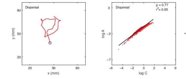
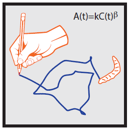
RM: First, the power law in question is the relationship between curvature and angular velocity that is observed when when a person traces out a line pattern on paper or when a fly larva traces out a path on the ground, as shown here:Â
<image.png>
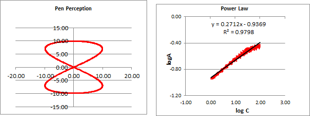
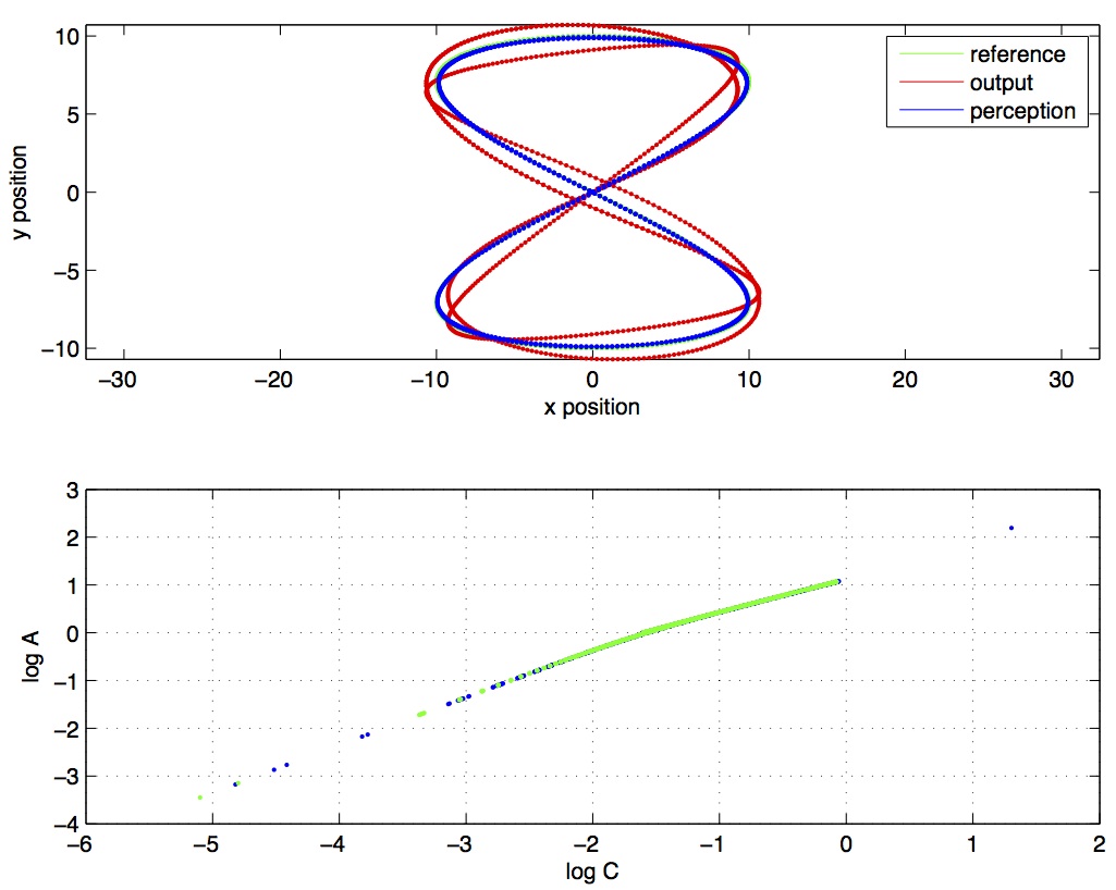
RM The equation in this figure is the power law relating angular velocity (A) to curvature (C) at each point on the pattern or path. I built a simple control model (using a spreadsheet) to simulate this behavior. The control model consisted of two control systems, each controlling a perception of the position of the tip of a pen; one system controlled the pen in the X dimension and the other controlled the position of the pen in the Y dimension. The reference inputs to each control system varied sinusoidally with frequencies adjusted so that the resulting pen movement pattern was a Lissajous pattern like the o
ne shown in the Figure on the left below. The Figure on the right is the power law relationship between curvature (C) and angular acceleration (A) produced by the control systems as they drew out the pattern on the left; a power law relationship between variables is a straight line when plotted in log-log coordinates.Â
<image.png>
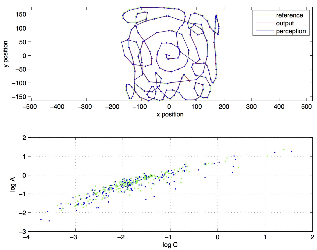
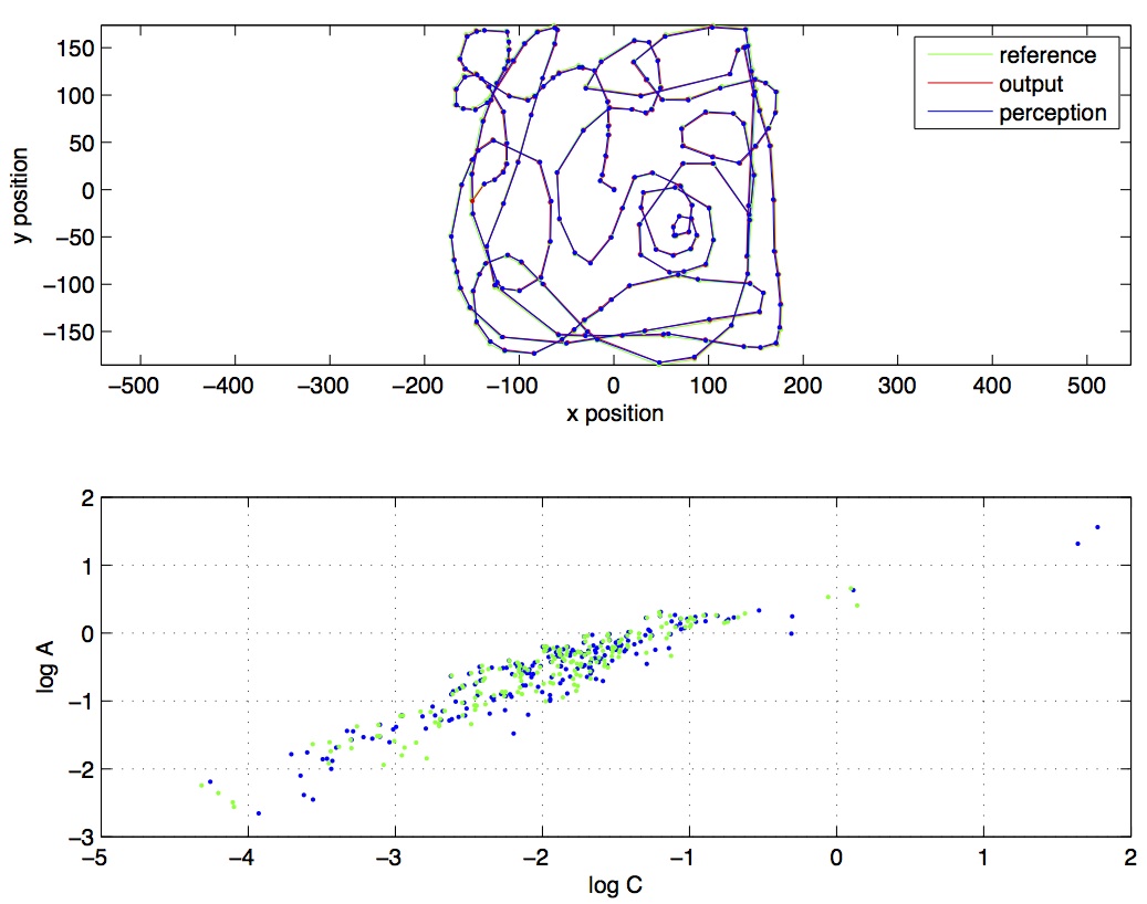
RM: The results of the simulation are rather remarkably similar to those found for the pattern of movement of the fly larva, as shown below. The Figure on the left is the path traced out by a fly larva, which consists of two circular paths, similar to the Lissajous pattern of pen movement in the simulation above. The Figure on the right is the power law relationship between curvature (C) and angular acceleration (A) produced by the control systems as they drew out the pattern on the left, again plott
ed in log-log coordinates.Â
<image.png>
RM: In both the real behavior and the simulation a power law fits the data very well: r2 > .95 in both cases. Also, in both cases the actual data point are slightly more bowed than the straight line defined by the power law. Finally, in both cases the data points don’t fall on a perfectly straight line; there is some variability in the points around the line. In the simulation, this spread of the data is created by adding a time varying disturbance to the movement of the pen; this disturbance, analogous to the varying resistance of the paper as you draw, is resisted by the control systems acting to keep the pen tip (the perception thereof) matching the time-varying reference for its position. The control systems resist these disturbances pretty well but not perfectly.Â
RM: This explanation of the power law relationship between angular velocity (A) and curvature (C) of motion requires no fancy assumptions about how neural output relates to muscle force or how muscle force relates to pen position. According to the model, the power relationship between A and C is an expected side effect of intentionally tracing out a curvy pattern or intentionally moving along a curvy path. It is not the inverse of the feedback function since many different feedback functions will produce the same result, as long as those functions allow control of the intended pattern or path.Â
RM: I say this is a trivially simple explanation because the model traces out the same pattern as does the real subject. So whatever relationship between A and C is found for a pattern produced by a a real living control system, the same relationship between A and C Â will be found for the pattern produced by the model to the extent
that the model produces the same pattern as the real system. The model does, however, explain the observed spread of points as a result of imperfect disturbance resistance.Â
RM: OK, let the criticisms begin. Oh, and I’ve attached the spreadsheet that I used to do this modeling exercise, if for no other reason than to show that I’m not making this stuff up;-)
BestÂ
Rick
–
Richard S. MarkenÂ
“The childhood of the human race is far from over. We
have a long way to go before most people will understand that what they do for
others is just as important to their well-being as what they do for
themselves.” – William T. Powers