Any ideas why or how “the control of perception” may give rise to this power law constraining geometry and kinematics in humans, and now in fruit fly larvae?
http://biorxiv.org/content/early/2016/07/05/062166
Thanks,
Alex
Any ideas why or how “the control of perception” may give rise to this power law constraining geometry and kinematics in humans, and now in fruit fly larvae?
http://biorxiv.org/content/early/2016/07/05/062166
Thanks,
Alex
Hi Alex, I hope I have the correct understanding of the law from my reading of the abstract, and I am sure other people must have proposed the explanation I have without knowing PCT, but tell me from what you know. I would assume that the adherence to the power law will be greater to the extent that the control of accuracy of the perceptual results of the curved movement is important for the animal (and therefore is controlled with high gain). In humans this could be asked about explicitly (‘how important was it for you to draw this exact shape’) or even manipulated (e.g. by comparing the adherence to the law when there are important consequences for the animal for being accurate or not accurate in terms of the shape drawn or in the target location the line ends up). In advanced animals and humans the law might be floughted during play, when the limits of control are meant to be overstepped within a safe context.
Has the speed/accuracy trade off idea been mentioned at all in the context of this law?
That’s my tupenny’s worth for now!
Warren
On 6 Jul 2016, at 15:33, Alex Gomez-Marin agomezmarin@gmail.com wrote:
Any ideas why or how “the control of perception” may give rise to this power law constraining geometry and kinematics in humans, and now in fruit fly larvae?
[http://biorxiv.org/content/early/2016/07/05/062166](Proofpoint Targeted Attack Protection
aQ&c=8hUWFZcy2Z-Za5rBPlktOQ&r=-dJBNItYEMOLt6aj_KjGi2LMO_Q8QB-ZzxIZIF8DGyQ&m=-OFy-JHbqmqjPN7VJIaj6uifem4QT5QpQEuzfCgF9XM&s=G9VeCsmdOa-YM0636O1vB6s11HQZlDpdXEdEbvGPD4k&e=)
Thanks,
Alex
In addition, I am thinking that the speed-curvature law should only hold up when the aim of the organism is to ultimately steer a path (of themselves or of a body part) to a target location. In this situation, the centrifugal force going outwards during the curve would have to be acted against as soon as a direction change is needed and as the force would be greater with speed it would pay to keep this speed low at higher curves. The exceptions in which the law would break down would be:
high speed is a goal (e.g. when engaged in high risk activities where loss of control is part of the goal - e.g. Jackass TV)
a fixed circular motion is a goal (e.g. when turning a wheel with a handle)
using the centrifugal force is a goal (e.g. when keeping water in bucket you spin fast in a vertical plane)
accuracy of the path is not important (e.g. scribbling at speed; not ‘doodling’ because a doodle has a desired aesthetic shape and so should be consistent with the law)
Some experiments there!
Warren
On Thu, Jul 7, 2016 at 4:26 AM, Warren Mansell wmansell@gmail.com wrote:
Hi Alex, I hope I have the correct understanding of the law from my reading of the abstract, and I am sure other people must have proposed the explanation I have without knowing PCT, but tell me from what you know. I would assume that the adherence to the power law will be greater to the extent that the control of accuracy of the perceptual results of the curved movement is important for the animal (and therefore is controlled with high gain). In humans this could be asked about explicitly (‘how important was it for you to draw this exact shape’) or even manipulated (e.g. by comparing the adherence to the law when there are important consequences for the animal for being accurate or not accurate in terms of the shape drawn or in the target location the line ends up). In advanced animals and humans the law might be floughted during play, when the limits of control are meant to be overstepped within a safe context.
Has the speed/accuracy trade off idea been mentioned at all in the context of this law?
That’s my tupenny’s worth for now!
Warren
On 6 Jul 2016, at 15:33, Alex Gomez-Marin agomezmarin@gmail.com wrote:
Any ideas why or how “the control of perception” may give rise to this power law constraining geometry and kinematics in humans, and now in fruit fly larvae?
Thanks,
Alex
–
Dr Warren Mansell
Reader in Clinical Psychology
School of Psychological Sciences
2nd Floor Zochonis Building
University of Manchester
Oxford Road
Manchester M13 9PL
Email: warren.mansell@manchester.ac.uk
Tel: +44 (0) 161 275 8589
Website: http://www.psych-sci.manchester.ac.uk/staff/131406
Advanced notice of a new transdiagnostic therapy manual, authored by Carey, Mansell & Tai - Principles-Based Counselling and Psychotherapy: A Method of Levels Approach
Available Now
Check www.pctweb.org for further information on Perceptual Control Theory
Thanks, Warren, for sharing your thoughts.Â
The power law has been described in humans and has been shown to be consistent with minimum jerk, thus suggesting that it results from smoothness.Â
The other question is how (some people claim cortical computations, other simple emergence in conjunction with biomechanical constraints).Â
For the fly larva it is quite clear that the animal is not thinking “I want to get from this point to precisely that point and I will do it through this path in order to minimize my jerk during the coming few seconds”. Yet, it is likely that evolution has shaped the larval system so that, in conjunction with the type of substrate it moves on, its particular body features, etc., the end result are trajectories that are somewhat optimal in the sense of the human trajectories.Â
For humans, it is quite shocking that one cannot break the law even if one tries to control of different variables: I wrote a matlab script that allows me to draw with my mouse on the screen and then calculate speed and curvature to immediately plot them in log-log. And I tried to “play” in order to generate trajectories whose speed-curvature did not comply with the law. And I couldn’t! (except for straight movements and stops, when curvature is zero and speed is zero).Â
So, regardless what the law means for the larva, it still presents an interesting puzzle in humans because changing my perceptions seems to be indifferent to this “motor control” principle.Â
That is why I was asking — to see if an explanation like the one Rick gave for the FFechner-Webber debate could help here.
On Thu, Jul 7, 2016 at 9:34 AM, Warren Mansell wmansell@gmail.com wrote:
In addition, I am thinking that the speed-curvature law should only hold up when the aim of the organism is to ultimately steer a path (of themselves or of a body part) to a target location. In this situation, the centrifugal force going outwards during the curve would have to be acted against as soon as a direction change is needed and as the force would be greater with speed it would pay to keep this speed low at higher curves. The exceptions in which the law would break down would be:Â
- achieving and maintaining a high speed in a curved path is more important to the organism than ultimately steering to a target or changing the curvature of the path to achieve another goal. This would occur to the degree that:
- high speed is a goal (e.g. when engaged in high risk activities where loss of control is part of the goal - e.g. Jackass TV)
- a fixed circular motion is a goal (e.g. when turning a wheel with a handle)
- using the centrifugal force is a goal (e.g. when keeping water in bucket you spin fast in a vertical plane)
- accuracy of the path is not important (e.g. scribbling at speed; not ‘doodling’ because a doodle has a desired aesthetic shape and so should be consistent with the law)
Some experiments there!
Warren
Â
On Thu, Jul 7, 2016 at 4:26 AM, Warren Mansell wmansell@gmail.com wrote:
Hi Alex, I hope I have the correct understanding of the law from my reading of the abstract, and I am sure other people must have proposed the explanation I have without knowing PCT, but tell me from what you know. I would assume that the adherence to the power law will be greater to the extent that the control of accuracy of the perceptual results of the curved movement is important for the animal (and therefore is controlled with high gain). In humans this could be asked about explicitly (‘how important was it for you to  draw this exact shape’) or even manipulated (e.g. by comparing the adherence to the law when there are important consequences for the animal for being accurate or not accurate in terms of the shape drawn or in the target location the line ends up). In advanced animals and humans the law might be floughted during play, when the limits of control are meant to be overstepped within a safe context.
Has the speed/accuracy trade off idea been mentioned at all in the context of this law?
That’s my tupenny’s worth for now!
Warren
On 6 Jul 2016, at 15:33, Alex Gomez-Marin agomezmarin@gmail.com wrote:
Any ideas why or how “the control of perception” may give rise to this power law constraining geometry and kinematics in humans, and now in fruit fly larvae?
Thanks,
Alex
–
Dr Warren Mansell
Reader in Clinical Psychology
School of Psychological Sciences
2nd Floor Zochonis Building
University of Manchester
Oxford Road
Manchester M13 9PL
Email: warren.mansell@manchester.ac.uk
Â
Tel: +44 (0) 161 275 8589
Â
Website: http://www.psych-sci.manchester.ac.uk/staff/131406
Â
Advanced notice of a new transdiagnostic therapy manual, authored by Carey, Mansell & Tai - Principles-Based Counselling and Psychotherapy: A Method of Levels Approach
Available Now
Check www.pctweb.org for further information on Perceptual Control Theory
That’s interesting and yes, of course, building a computer program is the way to test it. But I can draw a circle (consistent curvature) with my finger at variable speeds, so how does that work?
Warren
On Thu, Jul 7, 2016 at 9:34 AM, Warren Mansell wmansell@gmail.com wrote:
In addition, I am thinking that the speed-curvature law should only hold up when the aim of the organism is to ultimately steer a path (of themselves or of a body part) to a target location. In this situation, the centrifugal force going outwards during the curve would have to be acted against as soon as a direction change is needed and as the force would be greater with speed it would pay to keep this speed low at higher curves. The exceptions in which the law would break down would be:
- achieving and maintaining a high speed in a curved path is more important to the organism than ultimately steering to a target or changing the curvature of the path to achieve another goal. This would occur to the degree that:
- high speed is a goal (e.g. when engaged in high risk activities where loss of control is part of the goal - e.g. Jackass TV)
- a fixed circular motion is a goal (e.g. when turning a wheel with a handle)
- using the centrifugal force is a goal (e.g. when keeping water in bucket you spin fast in a vertical plane)
- accuracy of the path is not important (e.g. scribbling at speed; not ‘doodling’ because a doodle has a desired aesthetic shape and so should be consistent with the law)
Some experiments there!
Warren
On Thu, Jul 7, 2016 at 4:26 AM, Warren Mansell wmansell@gmail.com wrote:
Hi Alex, I hope I have the correct understanding of the law from my reading of the abstract, and I am sure other people must have proposed the explanation I have without knowing PCT, but tell me from what you know. I would assume that the adherence to the power law will be greater to the extent that the control of accuracy of the perceptual results of the curved movement is important for the animal (and therefore is controlled with high gain). In humans this could be asked about explicitly (‘how important was it for you to draw this exact shape’) or even manipulated (e.g. by comparing the adherence to the law when there are important consequences for the animal for being accurate or not accurate in terms of the shape drawn or in the target location the line ends up). In advanced animals and humans the law might be floughted during play, when the limits of control are meant to be overstepped within a safe context.
Has the speed/accuracy trade off idea been mentioned at all in the context of this law?
That’s my tupenny’s worth for now!
Warren
On 6 Jul 2016, at 15:33, Alex Gomez-Marin agomezmarin@gmail.com wrote:
Any ideas why or how “the control of perception” may give rise to this power law constraining geometry and kinematics in humans, and now in fruit fly larvae?
Thanks,
Alex
–
Dr Warren Mansell
Reader in Clinical Psychology
School of Psychological Sciences
2nd Floor Zochonis Building
University of Manchester
Oxford Road
Manchester M13 9PL
Email: warren.mansell@manchester.ac.uk
Tel: +44 (0) 161 275 8589
Website: http://www.psych-sci.manchester.ac.uk/staff/131406
Advanced notice of a new transdiagnostic therapy manual, authored by Carey, Mansell & Tai - Principles-Based Counselling and Psychotherapy: A Method of Levels Approach
Available Now
Check www.pctweb.org for further information on Perceptual Control Theory
Perhaps you could give an overview of what this speed curvature power law is, I’m not familiar with it?
                Rupert

                      On 6 July 2016 15:33:46
BST, Alex Gomez-Marin agomezmarin@gmail.com wrote:
Any ideas why or how “the control of perception” may give rise to this power law constraining geometry and kinematics in humans, and now in fruit fly larvae?
Thanks,
Alex
Regards,
Dr Rupert Young
–
Sent from my Android device with K-9 Mail. Please excuse my brevity.
Thanks for the interest.
Yes, you can draw a circle at whatever speed you want (within upper and lower limits, of course), but it turns out that the faster you draw the curve, the less curved you can can draw it, and the opposite.
That drawing movements accelerate and decelerate depending on what is actually being drawn at every point along the curve is a beautiful old result from 1893 (Sur la vitesse des mouvements graphiques, Travaux du Laboratoire de psychologie physiologique, R. Ph., 35, p. 664-671.).
In the 1980’s Lacquaniti and colleagues found that such proportionality relation follows a power law: speed = constant * curvature^(exponent). This means that plotting both geometric (curvature) and kinematic (speed) degrees of freedom in a log-log plot, they follow a straight line across orders of magnitude. And it is hardly escapable!: you draw on a piece of paper (or imagine your finger drawing in the air) and you think you could do it at any speed-curvature values, you are surprised to realize (specially if you can record your trajectory and calculate speed and curvature) that they indeed fall into that straight line in log-log space.
Read this short abstract and intro here.
This has been relatively well studied in human motor control literature, yet I haven’t found anyone asking what it means from the point of view of perception. Your views are really really suitable here.
On Fri, Jul 8, 2016 at 9:36 AM, rupert@perceptualrobots.com wrote:
Perhaps you could give an overview of what this speed curvature power law is, I’m not familiar with it?
Rupert
On 6 July 2016 15:33:46 BST, Alex Gomez-Marin agomezmarin@gmail.com wrote:
Any ideas why or how “the control of perception” may give rise to this power law constraining geometry and kinematics in humans, and now in fruit fly larvae?
Thanks,
Alex
Regards,
Dr Rupert Young
–
Sent from my Android device with K-9 Mail. Please excuse my brevity.
Hi Alex, it still seems to me that this should have something to do with centripetal force perpendicular to the momentary direction of movement, rather than muscles per se. See this http://m.phys.org/news/2016-04-science-remarkable-wall-death-motorcycle.html
On Fri, Jul 8, 2016 at 9:36 AM, rupert@perceptualrobots.com wrote:
Perhaps you could give an overview of what this speed curvature power law is, I’m not familiar with it?
Rupert
On 6 July 2016 15:33:46 BST, Alex Gomez-Marin agomezmarin@gmail.com wrote:
Any ideas why or how “the control of perception” may give rise to this power law constraining geometry and kinematics in humans, and now in fruit fly larvae?
Thanks,
Alex
Regards,
Dr Rupert Young
–
Sent from my Android device with K-9 Mail. Please excuse my brevity.
[Martin Taylor 2016.07.08.12.00]
I don't think this can be correct. Consider the inertia of the
crawling fruit fly larva, and the fact that it applies also when one
tries to draw in a viscous medium. Without having analyzed the
situation to my own satisfaction, my hypothesis is that it is likely
to have more to do with the speed of perception of rapidly changing
directions. I wonder if the same thing holds in more abstract spaces
that do not involve physical locations?
Incidentally, if you look at the power-law scatter-plots rather than
the fitted straight line, you can see that the power changes rather
dramatically and consistently between the lower and higher ends of
the plot. I haven’t tried to partition it numerically, but by eye, I
would say there could be a factor of two change in the exponent. I
think any explanation has to take that into account as well.
Furthermore, I wonder why they use the radius of curvature versus
the angular change in velocity rather than the linear along-track
velocity versus the angular velocity, which would seem a much more
natural relationship to consider?
Martin
On 2016/07/8 11:51 AM, Warren Mansell
wrote:
Hi Alex, it still seems to me that this should have somethingto do with centripetal force perpendicular to the momentary
direction of movement, rather than muscles per se. See this
On 8 Jul 2016, at 09:54, Alex Gomez-Marin < >wrote:
Thanksfor the interest.
Yes,you can draw a circle at whatever speed you want (within
upper and lower limits, of course), but it turns out
that the faster you draw the curve, the less curved you
can can draw it, and the opposite.
Thatdrawing movements accelerate and decelerate depending on
what is actually being drawn at every point along the
curve is a beautiful old result from 1893 (Sur la
vitesse des mouvements graphiques, Travaux du
Laboratoire de psychologie physiologique, R. Ph., 35, p.
664-671.).
Inthe 1980’s Lacquaniti and colleagues found that such
proportionality relation follows a power law: speed =
constant * curvature^(exponent). This means that
plotting both geometric (curvature) and kinematic
(speed) degrees of freedom in a log-log plot, they
follow a straight line across orders of magnitude. And
it is hardly escapable!: you draw on a piece of paper
(or imagine your finger drawing in the air) and you
think you could do it at any speed-curvature values, you
are surprised to realize (specially if you can record
your trajectory and calculate speed and curvature) that
they indeed fall into that straight line in log-log
space.
Read this short abstract and intro here.
Thishas been relatively well studied in human motor control
literature, yet I haven’t found anyone asking what it
means from the point of view of perception. Your views
are really really suitable here.
On Fri, Jul 8, 2016 at 9:36 AM, rupert@perceptualrobots.com
wrote:Perhaps you could give an overview of what thisspeed curvature power law is, I’m not familiar with
it?Rupert On 6 July 2016 15:33:46BST, Alex Gomez-Marin < >
wrote:
Regards,
                Dr Rupert Young

                [www.perceptualrobots.com](https://urldefense.proofpoint.com/v2/url?u=http-3A__www.perceptualrobots.com&d=CwMFaQ&c=8hUWFZcy2Z-Za5rBPlktOQ&r=-dJBNItYEMOLt6aj_KjGi2LMO_Q8QB-ZzxIZIF8DGyQ&m=u13yxGXNm47zqc5b0-h7ZLw7zz9mWIgeWDBAQTNsjhw&s=x7PTd7JMaJgGiZyEzQxWo6gbDpYuQ_n7cCwnKeQs7Fw&e=)

                    --

                    Sent from my Android device with K-9 Mail.
Please excuse my brevity.
http://m.phys.org/news/2016-04-science-remarkable-wall-death-motorcycle.htmlagomezmarin@gmail.com
Anyideas why or how “the control of
perception” may give rise to this power
law constraining geometry and kinematics
in humans, and now in fruit fly larvae?
Thanks,
Alex
[From Rick Marken (2016.07.08.1100)]
On Thu, Jul 7, 2016 at 2:52 PM, Alex Gomez-Marin agomezmarin@gmail.com wrote:
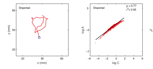
AGM: For humans, it is quite shocking that one cannot break the law even if one tries to control of different variables: I wrote a matlab script that allows me to draw with my mouse on the screen and then calculate speed and curvature to immediately plot them in log-log. And I tried to “play” in order to generate trajectories whose speed-curvature did not comply with the law. And I couldn’t! (except for straight movements and stops, when curvature is zero and speed is zero).Â
RM: That’s great Alex! Do your plots look like this:Â
RM: The relationship between curvature (C) and angular velocity (A) is, indeed, remarkably close to a perfect power relationship. But notice that there is also a very clear and consistent bow in the relationship. I’m no mathematician but what this suggests to me is that there is a very precise mathematical relationship between C and A that is only approximated – though very well approximated-- by the power law.
RM: The level of precision of the relationship between C and A suggests to me that it reflects a physical rather than a behavioral law. So my guess is that the observed approximate power law relating C to A is a reflection of the inverse of the feedback connection between output neural signals sent to the muscles that move the mouse, in the case of your demo) and input (perception of cursor position).Â
RM: You could test this hypothesis by simulating your own behavior in your demo using two simple control systems, one controlling the cursor in the X dimension and the other controlling the cursor in the Y dimension. The important part of the simulation would be putting in the correct physics of the feedback connection between simulated neural output and cursor movement; this would mainly have to take into account the physics of moving the mouse. The references to each control system would be the actual cursor movement that you produced on a previous run; that is, use the X and Y positions of the cursor over time as the time varying references for the X and Y dimension control systems, respectively.Â
AGM: That is why I was asking to see if an explanation like the one Rick gave for thee Fechner-Webber debate could help here.
RM: Actually, my hypothesized explanation is precisely the same as my explanation of the power function in psychophysics (I assume you are referring to my Behavioral Illusion paper – http://www.mindreadings.com/BehavioralIllusion.pdf -- which was reprinted in Doing Research on Purpose). In both cases I am saying that the observed relationship is the inverse of the feedback connection between output and input.Â
RM: I do hope you try this. Given that you are a physicist I think you will have no problem simulating the physics of the connection between neural output and visual input. And the control systems are very simple. And you’ve already got the program that plots the relationship between C and A.Â
RM: Of course, the inverse feedback function idea about the observed relationship between C and A is just a hypothesis; if the result of the simulation is that the relationship between C and A does’t look exactly like the one obtained for real organisms then the inverse of the feedback function is not the explanation, even though it seems so right. But that’s the fun (and pain) of science; you put all your cards on the table (with a precisely developed theoretical prediction) and see if nature “calls your bluff”, so to speak.Â
RM: I hope you do this simulation, Alex. If the “inverse feedback function” explanation pans out I’d love to write a paper on this with you. If it doesn’t pan out then we’ll have to think of an alternative explanation. Hopefully, if my suggested explanation does fail we can get hints about a better explanation by looking at how it failed.Â
RM: So do you think you can do the simulation Alex?
Best regards
Rick
Â
–
Richard S. MarkenÂ
“The childhood of the human race is far from over. We
have a long way to go before most people will understand that what they do for
others is just as important to their well-being as what they do for
themselves.” – William T. Powers
[From Rupert Young (2016.07.09 11.30)]
Does that mean then that you can draw an uppercase "O" faster than a
lowercase “o” (normalising for circumference)? I would have that
might be due to degrees of freedom of the hand relative the
orientation of the drawer. That is, if you draw a straight line,
from left to right there is only one degree of freedom involved, of
the twisting of the wrist. Whereas if you draw a curve it involves
moving the stylus towards the body which involves two degrees of
freedom, of moving the thumb and forefinger. It would make sense
that the latter is slower, and in PC T terms requires a coordinating
higher level.
I guess this could be tested by drawing a simple “+”. The
hypothesis being that it is slower to draw the vertical line than
the horizontal line; and requires two PCT levels. Regards,
Rupert
On 08/07/2016 09:54, Alex Gomez-Marin
wrote:
Yes,you can draw a circle at whatever speed you want (within upper
and lower limits, of course), but it turns out that the faster
you draw the curve, the less curved you can can draw it, and
the opposite.
Replies and ideas for Martin, **Rick,** Rupert and **Warren **below:
Overall, if we find some perceptual aspects of this motor control law, that would be something interesting to both worlds.
Martin, regarding your question for more abstract spaces, yes, the law has been shown not only in hand-writing but whole arm movements and also walking.
And yes, one can look more closely into the one-exponent fit and perhaps see more structure there. Also, there can be different intercept values in the regression, that is why it is important to do it per animal. In some cases, when animals/humans stop-and-go, one needs to analyze the speed-curvature relationship per trajectory segment. But this gets us into more complicated issues. Still, the law, with some corrections, applies there.
We use angular velocity (A=V/R) versus curvature (C=1/R) cause it is more convenient for the fit. Yet, one can test V-vs-R rather than A-vs-C and the law still works (with the corresponding exponent depending on the degrees of freedom considered).
Rick, good eye: there is a bow, which means that it is not mathematically obligatory to have the precise A(t)=kC(t)^beta relationship. Power laws, specially in biology and specially when estimated from real data, are always fits across several orders of magnitude, where points do not lie exactly on a straight line. So, yes, animals can slightly change their curvature for the same speed, and viceversa.
The power law obviously reflects physics, but it is not physics alone. It reflects an intrinsic aspect of the biology. Note that an inter system could break it. So, why does a living one follow it? Plus, note in the dots of the plots (every dot an individual fly), that very few, yet still a few animals do not follow it quite well, so it is not an obligatory outcome of physics.
Now, it can be that part of it stems from the feedback. Actually, I would say that is for sure: that the world is shaping the behavioral law. But, from this to proving that it is a behavioral illusion (thus, only the feedback), I think it is very unlikely, and perhaps even impossible to prove.Â
However, I would be happy either way, to prove it or not, because science is about finding out what is going on, whether you prefer it or not.
I will do the simulation. Still, some things need to be more explicit. The organism function is the typical linear decay function with the linear term as error, right? And, you propose that I use as disturbance my previous output trajectory? And what is the environment function (feedback connection), then? It is unclear to me how to simulate that cause there are missing bits.Â
Perhaps a similar interesting thing would be to draw an ellipse (people have been asked to draw ellipses by themselves and they do so following the power law) but now a dot is moving on that ellipse and the job of the human playing the demo is to either follow the dot or draw a mirror image or even keep a knot at the center like the rubber band task. That would be interesting because now we can program the dot to move at different speeds, and since the curvature is fixed, we would be asking the human playing the demo to control its perception so as to actually violate the law. And then learn what makes it hard to maintain that. Or change the feedback, or change the disturbance, etc.
Rupert, this means that, in general, the higher the local curvature of the drawing, the stronger the tendency to slow down the instantaneous velocity, and when plot over several orders of magnitude, the relation is a power function.
I like your comments about more than one degree of freedom. I don’t see why their control necessarily needs to happen at different levels in the hierarchy.Â
For the “+” experiment, note that in straight lines the law breaks down because curvature is formally infinite. So, it has to be for curved lines and non-zero velocity, which perhaps is related to your point of at least two degrees of freedom at work.
Warren, as you suggest different goals from the animal perspective, I was thinking that such perceptions should go really thru propioception, since it is quite unlikely that the larva uses visual cues (they can’t see much) to figure out optic flow, etc. so as to know how fast they are moving. They are essentially “local creatures”, so they can smell quite well, more or less phototax, all the rest being somatosensation. So, that is quite an interesting situation because the animal would need to kind of count its peristaltic waves and keep track of its body curvature to sense how fast and how curved in order to control it.Â
Still, there is the possibility that it is not controlling anything of this, but something else (what could that be?!) and that the “output” of that turns out to be such a curious non-trivial law.Â
Note that in principle a physical system should be able to break such geometry (curvature) — kinematics (sspeed) constraint, but that does not happen in biological movement.
Another point of intrigue is that dynamic effects (beyond geometry and kinematics) have been shown to modify the exponent in humans from 2/3 to 3/4, which is what we find in the fruit fly larva.
Thanks, guys, for this chain of inspiring thoughts!
Alex
On Sat, Jul 9, 2016 at 12:34 PM, Rupert Young rupert@perceptualrobots.com wrote:
[From Rupert Young (2016.07.09 11.30)]
On 08/07/2016 09:54, Alex Gomez-Marinwrote:
Yes,you can draw a circle at whatever speed you want (within upper
and lower limits, of course), but it turns out that the faster
you draw the curve, the less curved you can can draw it, and
the opposite.Â
Does that mean then that you can draw an uppercase "O" faster than alowercase “o” (normalising for circumference)? I would have that
might be due to degrees of freedom of the hand relative the
orientation of the drawer. That is, if you draw a straight line,
from left to right there is only one degree of freedom involved, of
the twisting of the wrist. Whereas if you draw a curve it involves
moving the stylus towards the body which involves two degrees of
freedom, of moving the thumb and forefinger. It would make sense
that the latter is slower, and in PC T terms requires a coordinating
higher level.I guess this could be tested by drawing a simple "+". Thehypothesis being that it is slower to draw the vertical line than
the horizontal line; and requires two PCT levels.Regards, Rupert
[Martin Taylor 2016.07.09.23.47]
Replies and ideas for Martin, Rick, Rupert and **Warren **below:
Overall, if we find some perceptual
aspects of this motor control law, that would be
something interesting to both worlds.
Martin , regarding your
question for more abstract spaces, yes, the law has been
shown not only in hand-writing but whole arm movements and
also walking.
I was thinking more of abstract
spaces such as hue. Hand-writing, whole-arm movements and walking
all involve physical motion in real space.
We use angular velocity (A=V/R)versus curvature (C=1/R) cause it is more convenient for
the fit. Yet, one can test V-vs-R rather than A-vs-C and
the law still works (with the corresponding exponent
depending on the degrees of freedom considered).
Yes. Different ways of looking at
it lead one to think of different possible perceptions that might
be being controlled. For example, given the same data, linear
velocity V = R^gamma where gamma = 1-Beta, so for a human in air,
roughly speaking V=R^0.3 and in water, or for the larva, V =
R^0.25 [read the = sign as “varies as”]. That makes me think of
how the future track will deviate from a Newtonian tangential
continuation of the track up to now. For the viscous movements, R
matters less than for the free-air movement. I don’t see that
relation when I think of A vs C, even though they both actually
say exactly the same thing. Whether this is significant, I know
not, but it would be consistent with a deeper “look-ahead” around
the curve’s deviation from the tangent in the low-viscosity
situation.
I give this only as an example of how different ways of expressing
the same data can lead one’s thoughts in different directions, not
as a proposed explanation for the observations.
Martin
Thanks Martin.
With respect to abstract spaces, the law has been found in dimensionality reduced neural movement related activity and also in speech, but I am not very familiar with that literature. However, the law is mainly for real space speed-curvature, and not an arbitrary spaces.
You are very right that although one can mathematically transform this quantity into another, the animal is presumably controlling this quantity and not another. So, good point!
On Sun, Jul 10, 2016 at 6:06 AM, Martin Taylor mmt-csg@mmtaylor.net wrote:
[Martin Taylor 2016.07.09.23.47]
Replies and ideas for Martin, Rick, Rupert and **Warren **below:
Overall, if we find some perceptual
aspects of this motor control law, that would be
something interesting to both worlds.
Martin , regarding your
question for more abstract spaces, yes, the law has been
shown not only in hand-writing but whole arm movements and
also walking.
I was thinking more of abstractspaces such as hue. Hand-writing, whole-arm movements and walking
all involve physical motion in real space.
We use angular velocity (A=V/R)versus curvature (C=1/R) cause it is more convenient for
the fit. Yet, one can test V-vs-R rather than A-vs-C and
the law still works (with the corresponding exponent
depending on the degrees of freedom considered).
Yes. Different ways of looking atit lead one to think of different possible perceptions that might
be being controlled. For example, given the same data, linear
velocity V = R^gamma where gamma = 1-Beta, so for a human in air,
roughly speaking V=R^0.3 and in water, or for the larva, V =
R^0.25 [read the = sign as “varies as”]. That makes me think of
how the future track will deviate from a Newtonian tangential
continuation of the track up to now. For the viscous movements, R
matters less than for the free-air movement. I don’t see that
relation when I think of A vs C, even though they both actually
say exactly the same thing. Whether this is significant, I know
not, but it would be consistent with a deeper “look-ahead” around
the curve’s deviation from the tangent in the low-viscosity
situation.I give this only as an example of how different ways of expressingthe same data can lead one’s thoughts in different directions, not
as a proposed explanation for the observations.Martin
[From Rick Marken (2016.07.10.1050)]
Hi Alex –
On Sat, Jul 9, 2016 at 9:30 AM, Alex Gomez-Marin agomezmarin@gmail.com wrote:
AGM: Rick, I will do the simulation. Still, some things need to be more explicit. The organism function is the typical linear decay function with the linear term as error, right? And, you propose that I use as disturbance my previous output trajectory? And what is the environment function (feedback connection), then? It is unclear to me how to simulate that cause there are missing bits.
RM: Great. Here’s my idea. Two control systems, one controlling the position of the pen in the X dimension and the other controlling the position of the pen in the Y dimension. So the controlled variables are p.x (X position of pen tip) and p.y (Y position of pen tip). The system equations for each system, written as computer replacement statements, might be:
o.x := o.x + slow.x * (gain.x*(r.x-p.x)-o.x) (1a)
o.y := o.y + slow.y * (gain.y*(r.y-p.y)-o.y) (1b)
RM: Here the outputs are proportional to a leaky integration of error, the difference between reference for (r.x and r.y) and perception of (p.x and p.y) the actual position of the pen tip. You can manually vary the values for the gain and slowing parameters to achieve stability; but slowing should be inversely related to gain; a reasonable start would be to set the gains at 50 and the slowing factors at .01.
RM: I see these outputs as forces that are continuously converted into new pen positions. Since acceleration of the pen tip is proportional to force I would compute the new pen position this way:
v.x= v.x + o.x/m (2a)
v.y = vy +o.y/m (2b)
RM: converting acceleration into velocity.
p.x = p.x + v.x (3a)
p.y = p.y + v.y (3b)
RM: converting velocity into position
RM: I believe these equations performs an approximation to the integration of force into position and closes the loop from perception to perception. . There are no disturbances shown in these equations although m (which I was taking as the constant mass of the pen) could possibly be varied to mimic the constantly changing resistance of the surface on which the pen moves.
RM: Since there is an integration in the environmental feedback function (equations 2 and 3 a & b) you may not need the integration in the system equations (1 a & b). So a simpler and better form of the system equations may be:
o.x := gain.x*(r.x-p.x) (1a’)
o.y := gain.y*(r.y-p.y) (1b’)
RM: In this case the gain probably can’t exceed 1.0 for stability; but the integration in the feedback function may increase the loop gain and give you pretty good control. I’ll fiddle around with this myself and see what works best.
RM: The time varying values of r.x and r.y in equations 1 a & b should be the time varying X and Y pen positions from a person (like you) doing this task. This would let you see if the curvature-angular acceleration relationship found for the model matches that for a real living control system doing the same thing.
RM: If you get this simulation to work it would be great if you could put it into a form that could be run by people (like me) who don’t have matlab on our computers. Actually, if you could send the code to Adam Matic he could turn this into a javascript demo in no time (if he’s got any time;-). I’d like to give it a try myself but I’m working on finishing up some consulting work and writing that damn paper for you;-)
Best regards
Rick
–
Richard S. Marken
“The childhood of the human race is far from over. We
have a long way to go before most people will understand that what they do for
others is just as important to their well-being as what they do for
themselves.” – William T. Powers
[From Rick Marken (2016.07.10.2100)]
On Sun, Jul 10, 2016 at 3:54 PM, Alex Gomez-Marin agomezmarin@gmail.com wrote:
AGM: I see, Rick. That’s interesting. So you propose an input-output system that linearly integrates the error between my own spatial trajectory and the actual trajectory of the pen, which is what the system input-output system indeed produces in terms of acceleration (multiplied by the mass, which is the only contribution from the environment), right? And to see if that would still respect the law? I will definitely try, and we can then evolve it from there. Nice!
RM: Sounds right. I’m checking my calculations right now in a spreadsheet and I need to know how you calculate A (angular velocity) and C (curvature) for each point on the X,Y trace. So if I have 1000 X, Y points, how to I calculate A and C for point 10, for example?
Best
Rick
–
On Sun, Jul 10, 2016 at 7:51 PM, Richard Marken rsmarken@gmail.com wrote:
[From Rick Marken (2016.07.10.1050)]
Hi Alex –
On Sat, Jul 9, 2016 at 9:30 AM, Alex Gomez-Marin agomezmarin@gmail.com wrote:
AGM: Rick, I will do the simulation. Still, some things need to be more explicit. The organism function is the typical linear decay function with the linear term as error, right? And, you propose that I use as disturbance my previous output trajectory? And what is the environment function (feedback connection), then? It is unclear to me how to simulate that cause there are missing bits.
RM: Great. Here’s my idea. Two control systems, one controlling the position of the pen in the X dimension and the other controlling the position of the pen in the Y dimension. So the controlled variables are p.x (X position of pen tip) and p.y (Y position of pen tip). The system equations for each system, written as computer replacement statements, might be:
o.x := o.x + slow.x * (gain.x*(r.x-p.x)-o.x) (1a)
o.y := o.y + slow.y * (gain.y*(r.y-p.y)-o.y) (1b)
RM: Here the outputs are proportional to a leaky integration of error, the difference between reference for (r.x and r.y) and perception of (p.x and p.y) the actual position of the pen tip. You can manually vary the values for the gain and slowing parameters to achieve stability; but slowing should be inversely related to gain; a reasonable start would be to set the gains at 50 and the slowing factors at .01.
RM: I see these outputs as forces that are continuously converted into new pen positions. Since acceleration of the pen tip is proportional to force I would compute the new pen position this way:
v.x= v.x + o.x/m (2a)
v.y = vy +o.y/m (2b)
RM: converting acceleration into velocity.
p.x = p.x + v.x (3a)
p.y = p.y + v.y (3b)
RM: converting velocity into position
RM: I believe these equations performs an approximation to the integration of force into position and closes the loop from perception to perception. . There are no disturbances shown in these equations although m (which I was taking as the constant mass of the pen) could possibly be varied to mimic the constantly changing resistance of the surface on which the pen moves.
RM: Since there is an integration in the environmental feedback function (equations 2 and 3 a & b) you may not need the integration in the system equations (1 a & b). So a simpler and better form of the system equations may be:
o.x := gain.x*(r.x-p.x) (1a’)
o.y := gain.y*(r.y-p.y) (1b’)
RM: In this case the gain probably can’t exceed 1.0 for stability; but the integration in the feedback function may increase the loop gain and give you pretty good control. I’ll fiddle around with this myself and see what works best.
RM: The time varying values of r.x and r.y in equations 1 a & b should be the time varying X and Y pen positions from a person (like you) doing this task. This would let you see if the curvature-angular acceleration relationship found for the model matches that for a real living control system doing the same thing.
RM: If you get this simulation to work it would be great if you could put it into a form that could be run by people (like me) who don’t have matlab on our computers. Actually, if you could send the code to Adam Matic he could turn this into a javascript demo in no time (if he’s got any time;-). I’d like to give it a try myself but I’m working on finishing up some consulting work and writing that damn paper for you;-)
Best regards
Rick
–
Richard S. Marken
“The childhood of the human race is far from over. We
have a long way to go before most people will understand that what they do for
others is just as important to their well-being as what they do for
themselves.” – William T. Powers
Richard S. Marken
“The childhood of the human race is far from over. We
have a long way to go before most people will understand that what they do for
others is just as important to their well-being as what they do for
themselves.” – William T. Powers
Rick,
Angular velocity is simply defined as the instantaneous change in movement direction (the trajectory dots have a certain angular direction, then you take the time derivative of that) and curvature by means of the tipical local expression (see here).
Note that there are other numerical ways of estimating such mathematical quantities (for instance, one could estimate angular velocity by dividing speed by the instantaneous radius of curvature; also, local curvature could be estimated by a least squares fit of circumferences at every point, rather than the first and second derivatives formula above). Also, one must be careful with the smoothing of the raw data (too little smoothing amplifies the noise when calculating first and second derivatives; too much smoothing introduces numerical artefacts). So, there is a little bit of “numerical implementation kitchen” here…
With respect to the systems of equations you propose, it is pretty interesting because when transforming your discretized version of the dynamics into proper dynamical equations, and when plugging the equation for q_0 into q_i (note that “the behavior” we want to examine here is q_i, the trajectory, rather than q_0, the force, which is cool) one gets an equation for q_i that is all linear but with 1st, 2nd and 3rd time derivatives, which could be where the traces of the minimum-jerk optimisation process lies. I’ll have to see how much further I can push the analytical manipulations before running as a simulation.
Also, if one includes friction in the feedback equation, one gets q0=m d^2/dt^2 q_i - gamma d/dt q_i, and so this means that somehow “m” should not matter (the system compensates for it somehow) but “gamma” should be determining the dynamical contribution to the geomtric-kinematic exponent, which is what we observe in the fruit fly and our collaborators have seen in humans drawing ellipses in water. We’l see.
Check this paper out:
http://www.pnas.org/content/112/29/E3950.full
Final comment, even if we can prove that the behavior of the simulated system also has speed-curvature constraints in the form of a power law, that still does not explain where the power-law is emerging from since the simulated system is trying to follow the reference that we impose, which already has the speed-curvature constraints. I wonder whether there is a way to make the system dynamically autonomous, namely, to imagine a high-level reference that is dictating a path but not at which speed it must be drawn, and then let the system take that reference and control its perception so as to precisely produce the power law. That would be fantastic because we could should how such motor control optimality principles emerge from simply perceptual control dynamics.
Alex
On Mon, Jul 11, 2016 at 6:03 AM, Richard Marken rsmarken@gmail.com wrote:
[From Rick Marken (2016.07.10.2100)]
On Sun, Jul 10, 2016 at 3:54 PM, Alex Gomez-Marin agomezmarin@gmail.com wrote:
AGM: I see, Rick. That’s interesting. So you propose an input-output system that linearly integrates the error between my own spatial trajectory and the actual trajectory of the pen, which is what the system input-output system indeed produces in terms of acceleration (multiplied by the mass, which is the only contribution from the environment), right? And to see if that would still respect the law? I will definitely try, and we can then evolve it from there. Nice!
RM: Sounds right. I’m checking my calculations right now in a spreadsheet and I need to know how you calculate A (angular velocity) and C (curvature) for each point on the X,Y trace. So if I have 1000 X, Y points, how to I calculate A and C for point 10, for example?
Best
Rick
–
Richard S. Marken
“The childhood of the human race is far from over. We
have a long way to go before most people will understand that what they do for
others is just as important to their well-being as what they do for
themselves.” – William T. Powers
On Sun, Jul 10, 2016 at 7:51 PM, Richard Marken rsmarken@gmail.com wrote:
[From Rick Marken (2016.07.10.1050)]
Hi Alex –
On Sat, Jul 9, 2016 at 9:30 AM, Alex Gomez-Marin agomezmarin@gmail.com wrote:
AGM: Rick, I will do the simulation. Still, some things need to be more explicit. The organism function is the typical linear decay function with the linear term as error, right? And, you propose that I use as disturbance my previous output trajectory? And what is the environment function (feedback connection), then? It is unclear to me how to simulate that cause there are missing bits.
RM: Great. Here’s my idea. Two control systems, one controlling the position of the pen in the X dimension and the other controlling the position of the pen in the Y dimension. So the controlled variables are p.x (X position of pen tip) and p.y (Y position of pen tip). The system equations for each system, written as computer replacement statements, might be:
o.x := o.x + slow.x * (gain.x*(r.x-p.x)-o.x) (1a)
o.y := o.y + slow.y * (gain.y*(r.y-p.y)-o.y) (1b)
RM: Here the outputs are proportional to a leaky integration of error, the difference between reference for (r.x and r.y) and perception of (p.x and p.y) the actual position of the pen tip. You can manually vary the values for the gain and slowing parameters to achieve stability; but slowing should be inversely related to gain; a reasonable start would be to set the gains at 50 and the slowing factors at .01.
RM: I see these outputs as forces that are continuously converted into new pen positions. Since acceleration of the pen tip is proportional to force I would compute the new pen position this way:
v.x= v.x + o.x/m (2a)
v.y = vy +o.y/m (2b)
RM: converting acceleration into velocity.
p.x = p.x + v.x (3a)
p.y = p.y + v.y (3b)
RM: converting velocity into position
RM: I believe these equations performs an approximation to the integration of force into position and closes the loop from perception to perception. . There are no disturbances shown in these equations although m (which I was taking as the constant mass of the pen) could possibly be varied to mimic the constantly changing resistance of the surface on which the pen moves.
RM: Since there is an integration in the environmental feedback function (equations 2 and 3 a & b) you may not need the integration in the system equations (1 a & b). So a simpler and better form of the system equations may be:
o.x := gain.x*(r.x-p.x) (1a’)
o.y := gain.y*(r.y-p.y) (1b’)
RM: In this case the gain probably can’t exceed 1.0 for stability; but the integration in the feedback function may increase the loop gain and give you pretty good control. I’ll fiddle around with this myself and see what works best.
RM: The time varying values of r.x and r.y in equations 1 a & b should be the time varying X and Y pen positions from a person (like you) doing this task. This would let you see if the curvature-angular acceleration relationship found for the model matches that for a real living control system doing the same thing.
RM: If you get this simulation to work it would be great if you could put it into a form that could be run by people (like me) who don’t have matlab on our computers. Actually, if you could send the code to Adam Matic he could turn this into a javascript demo in no time (if he’s got any time;-). I’d like to give it a try myself but I’m working on finishing up some consulting work and writing that damn paper for you;-)
Best regards
Rick
–
Richard S. Marken
“The childhood of the human race is far from over. We
have a long way to go before most people will understand that what they do for
others is just as important to their well-being as what they do for
themselves.” – William T. Powers
And find two of the first papers on the subject, which already give a lot of hints of what may be going on from the subjects perspective.
Viviani1982.pdf (1.14 MB)
Lacquaniti19831.pdf (1.49 MB)
On Mon, Jul 11, 2016 at 11:22 AM, Alex Gomez-Marin agomezmarin@gmail.com wrote:
Rick,
Angular velocity is simply defined as the instantaneous change in movement direction (the trajectory dots have a certain angular direction, then you take the time derivative of that) and curvature by means of the tipical local expression (see here).
Note that there are other numerical ways of estimating such mathematical quantities (for instance, one could estimate angular velocity by dividing speed by the instantaneous radius of curvature; also, local curvature could be estimated by a least squares fit of circumferences at every point, rather than the first and second derivatives formula above). Also, one must be careful with the smoothing of the raw data (too little smoothing amplifies the noise when calculating first and second derivatives; too much smoothing introduces numerical artefacts). So, there is a little bit of “numerical implementation kitchen” here…
With respect to the systems of equations you propose, it is pretty interesting because when transforming your discretized version of the dynamics into proper dynamical equations, and when plugging the equation for q_0 into q_i (note that “the behavior” we want to examine here is q_i, the trajectory, rather than q_0, the force, which is cool) one gets an equation for q_i that is all linear but with 1st, 2nd and 3rd time derivatives, which could be where the traces of the minimum-jerk optimisation process lies. I’ll have to see how much further I can push the analytical manipulations before running as a simulation.
Also, if one includes friction in the feedback equation, one gets q0=m d^2/dt^2 q_i - gamma d/dt q_i, and so this means that somehow “m” should not matter (the system compensates for it somehow) but “gamma” should be determining the dynamical contribution to the geomtric-kinematic exponent, which is what we observe in the fruit fly and our collaborators have seen in humans drawing ellipses in water. We’l see.
Check this paper out:
Final comment, even if we can prove that the behavior of the simulated system also has speed-curvature constraints in the form of a power law, that still does not explain where the power-law is emerging from since the simulated system is trying to follow the reference that we impose, which already has the speed-curvature constraints. I wonder whether there is a way to make the system dynamically autonomous, namely, to imagine a high-level reference that is dictating a path but not at which speed it must be drawn, and then let the system take that reference and control its perception so as to precisely produce the power law. That would be fantastic because we could should how such motor control optimality principles emerge from simply perceptual control dynamics.
Alex
On Mon, Jul 11, 2016 at 6:03 AM, Richard Marken rsmarken@gmail.com wrote:
[From Rick Marken (2016.07.10.2100)]
On Sun, Jul 10, 2016 at 3:54 PM, Alex Gomez-Marin agomezmarin@gmail.com wrote:
AGM: I see, Rick. That’s interesting. So you propose an input-output system that linearly integrates the error between my own spatial trajectory and the actual trajectory of the pen, which is what the system input-output system indeed produces in terms of acceleration (multiplied by the mass, which is the only contribution from the environment), right? And to see if that would still respect the law? I will definitely try, and we can then evolve it from there. Nice!
RM: Sounds right. I’m checking my calculations right now in a spreadsheet and I need to know how you calculate A (angular velocity) and C (curvature) for each point on the X,Y trace. So if I have 1000 X, Y points, how to I calculate A and C for point 10, for example?
Best
Rick
–
Richard S. Marken
“The childhood of the human race is far from over. We
have a long way to go before most people will understand that what they do for
others is just as important to their well-being as what they do for
themselves.” – William T. Powers
On Sun, Jul 10, 2016 at 7:51 PM, Richard Marken rsmarken@gmail.com wrote:
[From Rick Marken (2016.07.10.1050)]
Hi Alex –
On Sat, Jul 9, 2016 at 9:30 AM, Alex Gomez-Marin agomezmarin@gmail.com wrote:
AGM: Rick, I will do the simulation. Still, some things need to be more explicit. The organism function is the typical linear decay function with the linear term as error, right? And, you propose that I use as disturbance my previous output trajectory? And what is the environment function (feedback connection), then? It is unclear to me how to simulate that cause there are missing bits.
RM: Great. Here’s my idea. Two control systems, one controlling the position of the pen in the X dimension and the other controlling the position of the pen in the Y dimension. So the controlled variables are p.x (X position of pen tip) and p.y (Y position of pen tip). The system equations for each system, written as computer replacement statements, might be:
o.x := o.x + slow.x * (gain.x*(r.x-p.x)-o.x) (1a)
o.y := o.y + slow.y * (gain.y*(r.y-p.y)-o.y) (1b)
RM: Here the outputs are proportional to a leaky integration of error, the difference between reference for (r.x and r.y) and perception of (p.x and p.y) the actual position of the pen tip. You can manually vary the values for the gain and slowing parameters to achieve stability; but slowing should be inversely related to gain; a reasonable start would be to set the gains at 50 and the slowing factors at .01.
RM: I see these outputs as forces that are continuously converted into new pen positions. Since acceleration of the pen tip is proportional to force I would compute the new pen position this way:
v.x= v.x + o.x/m (2a)
v.y = vy +o.y/m (2b)
RM: converting acceleration into velocity.
p.x = p.x + v.x (3a)
p.y = p.y + v.y (3b)
RM: converting velocity into position
RM: I believe these equations performs an approximation to the integration of force into position and closes the loop from perception to perception. . There are no disturbances shown in these equations although m (which I was taking as the constant mass of the pen) could possibly be varied to mimic the constantly changing resistance of the surface on which the pen moves.
RM: Since there is an integration in the environmental feedback function (equations 2 and 3 a & b) you may not need the integration in the system equations (1 a & b). So a simpler and better form of the system equations may be:
o.x := gain.x*(r.x-p.x) (1a’)
o.y := gain.y*(r.y-p.y) (1b’)
RM: In this case the gain probably can’t exceed 1.0 for stability; but the integration in the feedback function may increase the loop gain and give you pretty good control. I’ll fiddle around with this myself and see what works best.
RM: The time varying values of r.x and r.y in equations 1 a & b should be the time varying X and Y pen positions from a person (like you) doing this task. This would let you see if the curvature-angular acceleration relationship found for the model matches that for a real living control system doing the same thing.
RM: If you get this simulation to work it would be great if you could put it into a form that could be run by people (like me) who don’t have matlab on our computers. Actually, if you could send the code to Adam Matic he could turn this into a javascript demo in no time (if he’s got any time;-). I’d like to give it a try myself but I’m working on finishing up some consulting work and writing that damn paper for you;-)
Best regards
Rick
–
Richard S. Marken
“The childhood of the human race is far from over. We
have a long way to go before most people will understand that what they do for
others is just as important to their well-being as what they do for
themselves.” – William T. Powers
And you will NOT like this explanation based on modeling limb dynamics and muscle mechanics, which, if we could complement by control of perception, would quite illuminate the issue.
On Mon, Jul 11, 2016 at 12:43 PM, Alex Gomez-Marin agomezmarin@gmail.com wrote:
And find two of the first papers on the subject, which already give a lot of hints of what may be going on from the subjects perspective.
On Mon, Jul 11, 2016 at 11:22 AM, Alex Gomez-Marin agomezmarin@gmail.com wrote:
Rick,
Angular velocity is simply defined as the instantaneous change in movement direction (the trajectory dots have a certain angular direction, then you take the time derivative of that) and curvature by means of the tipical local expression (see here).
Note that there are other numerical ways of estimating such mathematical quantities (for instance, one could estimate angular velocity by dividing speed by the instantaneous radius of curvature; also, local curvature could be estimated by a least squares fit of circumferences at every point, rather than the first and second derivatives formula above). Also, one must be careful with the smoothing of the raw data (too little smoothing amplifies the noise when calculating first and second derivatives; too much smoothing introduces numerical artefacts). So, there is a little bit of “numerical implementation kitchen” here…
With respect to the systems of equations you propose, it is pretty interesting because when transforming your discretized version of the dynamics into proper dynamical equations, and when plugging the equation for q_0 into q_i (note that “the behavior” we want to examine here is q_i, the trajectory, rather than q_0, the force, which is cool) one gets an equation for q_i that is all linear but with 1st, 2nd and 3rd time derivatives, which could be where the traces of the minimum-jerk optimisation process lies. I’ll have to see how much further I can push the analytical manipulations before running as a simulation.
Also, if one includes friction in the feedback equation, one gets q0=m d^2/dt^2 q_i - gamma d/dt q_i, and so this means that somehow “m” should not matter (the system compensates for it somehow) but “gamma” should be determining the dynamical contribution to the geomtric-kinematic exponent, which is what we observe in the fruit fly and our collaborators have seen in humans drawing ellipses in water. We’l see.
Check this paper out:
Final comment, even if we can prove that the behavior of the simulated system also has speed-curvature constraints in the form of a power law, that still does not explain where the power-law is emerging from since the simulated system is trying to follow the reference that we impose, which already has the speed-curvature constraints. I wonder whether there is a way to make the system dynamically autonomous, namely, to imagine a high-level reference that is dictating a path but not at which speed it must be drawn, and then let the system take that reference and control its perception so as to precisely produce the power law. That would be fantastic because we could should how such motor control optimality principles emerge from simply perceptual control dynamics.
Alex
On Mon, Jul 11, 2016 at 6:03 AM, Richard Marken rsmarken@gmail.com wrote:
[From Rick Marken (2016.07.10.2100)]
On Sun, Jul 10, 2016 at 3:54 PM, Alex Gomez-Marin agomezmarin@gmail.com wrote:
AGM: I see, Rick. That’s interesting. So you propose an input-output system that linearly integrates the error between my own spatial trajectory and the actual trajectory of the pen, which is what the system input-output system indeed produces in terms of acceleration (multiplied by the mass, which is the only contribution from the environment), right? And to see if that would still respect the law? I will definitely try, and we can then evolve it from there. Nice!
RM: Sounds right. I’m checking my calculations right now in a spreadsheet and I need to know how you calculate A (angular velocity) and C (curvature) for each point on the X,Y trace. So if I have 1000 X, Y points, how to I calculate A and C for point 10, for example?
Best
Rick
–
Richard S. Marken
“The childhood of the human race is far from over. We
have a long way to go before most people will understand that what they do for
others is just as important to their well-being as what they do for
themselves.” – William T. Powers
On Sun, Jul 10, 2016 at 7:51 PM, Richard Marken rsmarken@gmail.com wrote:
[From Rick Marken (2016.07.10.1050)]
Hi Alex –
On Sat, Jul 9, 2016 at 9:30 AM, Alex Gomez-Marin agomezmarin@gmail.com wrote:
AGM: Rick, I will do the simulation. Still, some things need to be more explicit. The organism function is the typical linear decay function with the linear term as error, right? And, you propose that I use as disturbance my previous output trajectory? And what is the environment function (feedback connection), then? It is unclear to me how to simulate that cause there are missing bits.
RM: Great. Here’s my idea. Two control systems, one controlling the position of the pen in the X dimension and the other controlling the position of the pen in the Y dimension. So the controlled variables are p.x (X position of pen tip) and p.y (Y position of pen tip). The system equations for each system, written as computer replacement statements, might be:
o.x := o.x + slow.x * (gain.x*(r.x-p.x)-o.x) (1a)
o.y := o.y + slow.y * (gain.y*(r.y-p.y)-o.y) (1b)
RM: Here the outputs are proportional to a leaky integration of error, the difference between reference for (r.x and r.y) and perception of (p.x and p.y) the actual position of the pen tip. You can manually vary the values for the gain and slowing parameters to achieve stability; but slowing should be inversely related to gain; a reasonable start would be to set the gains at 50 and the slowing factors at .01.
RM: I see these outputs as forces that are continuously converted into new pen positions. Since acceleration of the pen tip is proportional to force I would compute the new pen position this way:
v.x= v.x + o.x/m (2a)
v.y = vy +o.y/m (2b)
RM: converting acceleration into velocity.
p.x = p.x + v.x (3a)
p.y = p.y + v.y (3b)
RM: converting velocity into position
RM: I believe these equations performs an approximation to the integration of force into position and closes the loop from perception to perception. . There are no disturbances shown in these equations although m (which I was taking as the constant mass of the pen) could possibly be varied to mimic the constantly changing resistance of the surface on which the pen moves.
RM: Since there is an integration in the environmental feedback function (equations 2 and 3 a & b) you may not need the integration in the system equations (1 a & b). So a simpler and better form of the system equations may be:
o.x := gain.x*(r.x-p.x) (1a’)
o.y := gain.y*(r.y-p.y) (1b’)
RM: In this case the gain probably can’t exceed 1.0 for stability; but the integration in the feedback function may increase the loop gain and give you pretty good control. I’ll fiddle around with this myself and see what works best.
RM: The time varying values of r.x and r.y in equations 1 a & b should be the time varying X and Y pen positions from a person (like you) doing this task. This would let you see if the curvature-angular acceleration relationship found for the model matches that for a real living control system doing the same thing.
RM: If you get this simulation to work it would be great if you could put it into a form that could be run by people (like me) who don’t have matlab on our computers. Actually, if you could send the code to Adam Matic he could turn this into a javascript demo in no time (if he’s got any time;-). I’d like to give it a try myself but I’m working on finishing up some consulting work and writing that damn paper for you;-)
Best regards
Rick
–
Richard S. Marken
“The childhood of the human race is far from over. We
have a long way to go before most people will understand that what they do for
others is just as important to their well-being as what they do for
themselves.” – William T. Powers
[From MK (2016.07.11.1505 CET)]
Do the trajectories "generated" by the virtual agents in the Crowd
demonstration conform to the described relationship?
M