Well it’s a good job I know you well Rick! ![]()
![]()
The thing I like about this model is that the inner cursor position loop is receiving a reference signal from the oscillator - it is following an oscillating reference, and this reference is phase-advanced and size-modulated, so that the resulting cursor movement always follows the size and phase of the target.
The additional benefit of that inner loop is low-pass filtering, and resistance to noise applied to the cursor.
Of course, the model could be reorganized, and things tumbled around, as I mentioned before. The final arbiter is experiment.
Good. The power law is not a side effect of only controlling the phase difference. It is a side effect of the system that is controlling, in this case, phase and size differences, and is also acting as a low-pass filter, and is also following a fast elliptical target.
The intended effect of the system is folowing the rhythm of the target and drawing the elliptic shape pattern of the correct size. At low average speeds (low frequency), the instantaneous cursor speed will match the target speed, it can go in any pattern. At high average speeds, the instantaneous speed will NOT follow the target speed. Instead, because of low-pass filtering, it will always be a pure sinusoid, and if you have an ellipse made of two pure sinusoids in x and y, they will fit the power law with the exponent of -1/3.
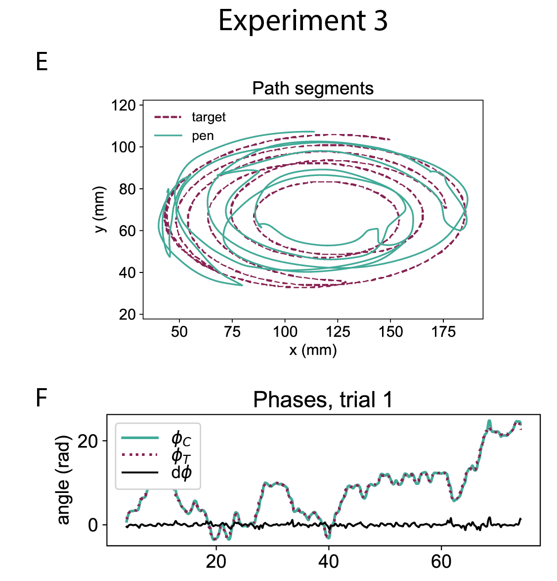
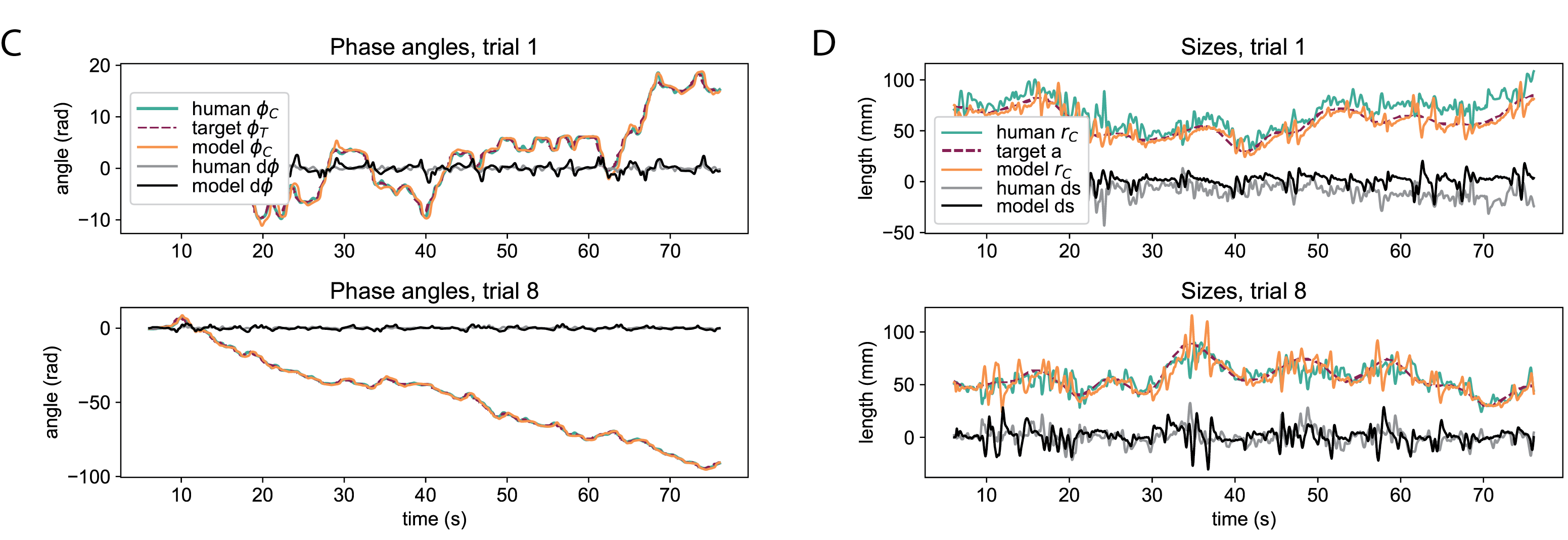
This is visible in human tracking:

And the model replicates this behavior:
No, this is wrong. You can make a perfect elliptic path with very different power law trajectories, or without any power law, and I have all of them. Look at the target trajectories in the two figures above. Perfect ellipse with constant speed has beta=0, with slight slowing down has beta=-1/3, and high slowing down is beta = -2/3. The model reproduces human behavior.
I also had an elliptic path target with random changes in phase and random changes in size and the model replicated human behavior.
Human:
Model:
How about reading the paper?
It looks like it’s receiving the reference from the difference between cursor and target measures in terms of the difference in their phase and size. Is this the “oscillator” you’re talking about or is there an actual oscillator involved? I don’t see one in the diagram of the model.
It’s difficult to tell what’s going on in that inner loop. It looks like that loop is controlling a variable, x.dot, that is being added to the the current cursor position, c,x. The noise seems to be added to x.dot, not to c.x. If your subject is moving the cursor with a mouse or joystick then what the inner loop is doing is controlling the position of that mouse or joystick, protecting it from noise disturbances, which is a filtering process. But the filtering (in the model) is of x.dot, the output that affects the cursor, c.x, not the cursor movement itself.
By the way, in the paper you mention that you low-pass filtered the subject data for analysis. Did you compare the model to the filtered or raw subject data? I’ve found that I have to filter the subject data for analysis or the data has too many invalid data points due to brief segments in the movement where the cursor moves in a straight line.
Yes, of course, such as planetary orbits.
Beautiful! Exactly what I would expect. If you do the regression and include the affine velocity variable – Af = X.dotY.dot.dot - Y.dotX.dot.dot – as a predictor you will see that the coefficient for the C predictor will be exactly -1/3 and for the Af predictor it will be exactly 1/3. And the R^2 for the regression will be 1.0.
This means that the degree to which you find a “power law” conforming coefficient for the relationship between V and C for any curved movement depends on the degree to which variations in Af are correlated with variations in C; the closer this correlation is to 0, the closer the power coefficient will be to its “lawful” value, -1/3. Since we typically find the power law coefficient to be about -1/3 plus or minus 1/7 for movements made by living systems, the interesting question to me seems to be what limits organisms to movements where Af has a low correlation with C.
How about presenting it at the IAPCT conference?
RSM
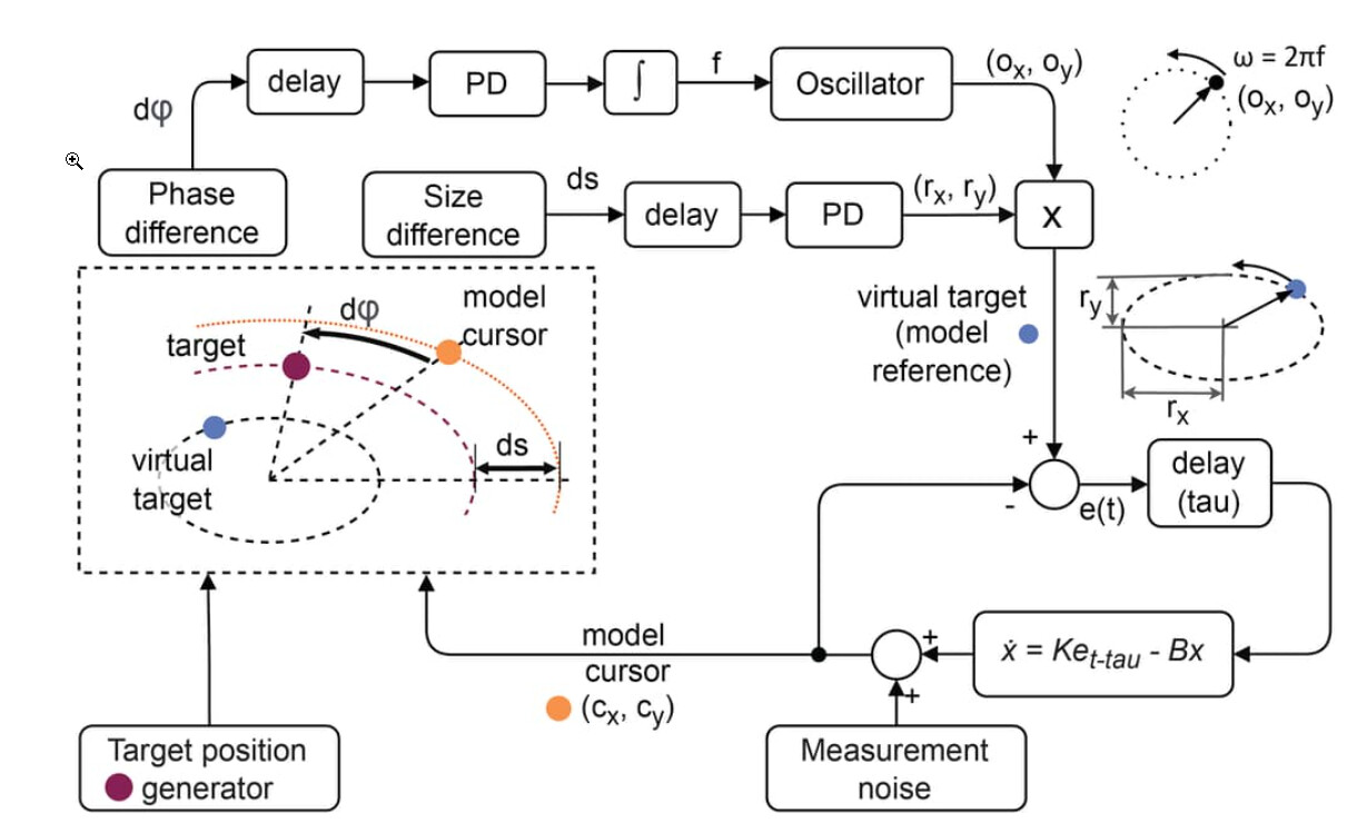
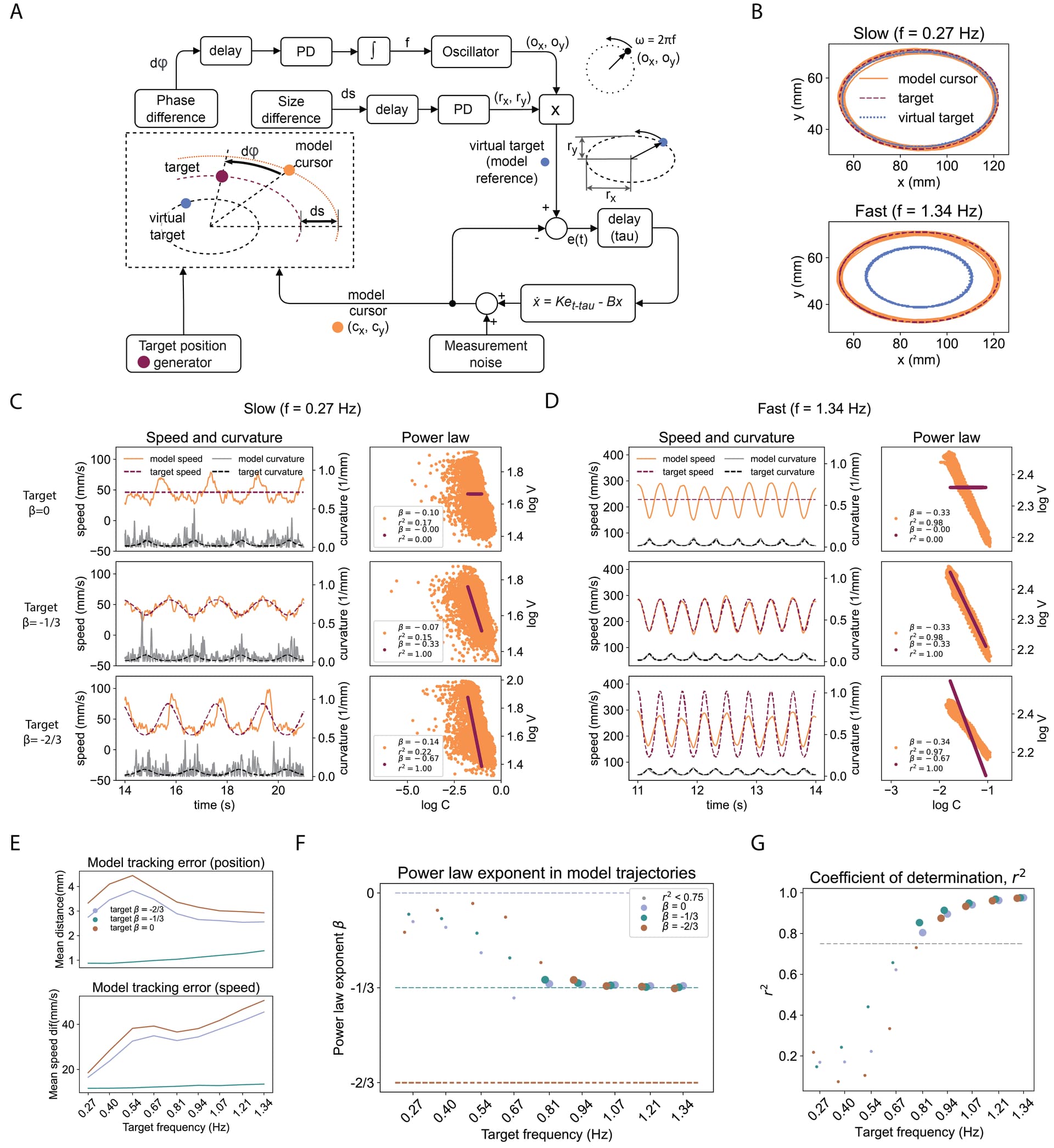
Look at the phase difference pathway. The phase difference (d-phi) is delayed, then there is proportional-derivative (PD box) controller, with implicit reference of zero radians. This error is integrated - variable f is the integral of the error. This f is the input to the harmonic 2D oscillator, you can recognize it by the labeled “Oscillator”. The frequency of the oscillator will be equal to f. The output is shown graphically as a spinning vector with coordinates (ox, oy). The length of the vector is always 1, so it is always going in a circle, sometimes slower, sometimes faster.
This is somewhat similar to a very old feedback called a phase-locked loop (PLL) used initially for demodulating radiowaves and whatnot, and today for synchronizing different signals. It is pretty much everywhere Phase-locked loop - Wikipedia
As a side-effect of controlling the phase distance, the frequecies of this oscillator and the target will be the same, the phase distance simply needs to be constant. Like, you can drive side-by-side to another car, or you can drive constant 50 meters behind, as a side-effect of controlling position, your speeds will match. Same thing with phase difference and frequency.
So, we have a signal synchronized to the target
Next, the size difference pathway: the variable ds is at every moment representing the difference between the sizes of the target-drawn ellipse, and the cursor drawn ellipse. The size is perceived as the width of the ellipse passing through the cursor, with the same center and same eccentricity as the target-drawn ellipse. This can handle large delays and still control the size pretty good.
The size difference is delayed and passed to a PD controller. There are two outputs, radius x, and radius y (rx and ry), and these are always in the same relationship so that the ellipse does not change eccentricity. rx and ry are multiplied (the box with the label X) by the oscillator output to create the reference signal. The reference will have the same angular position as the oscillator output, but will be stretched just enough to make the cursor move at the same size of the ellipse as the target.
Generally, this reference is going to be a bit in front of the target, so that the cursor could be exactly on the target. The cursor is not tracking the target, it is tracking the reference (or virtual target).
The inner loop has a shorthand expression for leaky integration, the output is x, not xdot:
xdot = K * e(t-tau) - Bx
In the code, this is:
x = x + xdot*dt
When the noise is added to x (simulating measurement noise in the tablet pen), this becomes cursor position C(cx, cy). The small black circle means “copy of the signal”. The inner loop is controlling cursor position, not in relation to the presented target, but in relation to the reference, or virtual target.
Filtered.
Not really, the -1/3 is just in ellipses. Other shapes have different exponents, depending on speed also.
Well, I finally read your paper, Adam. It’s quite good. You certainly used the appropriate methodology to study how movements are produced: testing for controlled variables and modeling.
My conclusion from the results is probably somewhat different than yours. I think it shows that the -1/3 power law is an irrelevant side effect that can be replicated only under certain circumstances (such as tracking a fast moving elliptical target). This is just like the word “hello” in Bill’s demo, with which I’m sure you are familiar, which can be replicated only with a two dimensional disturbance that is the mirror of “hello”.
I call the power law an “irrelevant side effect” of control because it was not the observation of that law that led you to your successful model; it was the observation of the variables being controlling in the movement. Once you identified the best candidates for controlled variables and incorporated them into a model that successfully replicated the human movements then you got the same -1/3 power law that was a side effect of the human movement. It’s your understanding of Power’s application of control theory to behavior that let you correctly model the movement behavior, not your understanding power law.
I think what you have discovered in this research is that moving in regular patterns, like an ellipse, involved control of a higher order variable – in this case the control of the delayed phase and size difference that results in phase locking – as well as well as control of a lower level variable: cursor position. You can test the two level nature of the controlling going on by adding a disturbance directly to the cursor and look for lack of correlation between the disturbance (dx, dy) and the cursor position (cx, cy). You may have done this already but I don’t recall seeing it in the paper.
Oh, I’m so honored. Maybe try leading with that before commenting on a paper, instead of wasting everyones time by skimming it and expressing strong opinions.
You’re really hamfisting the whole “I was right all allong” narrative. The whole point of the project was to find out when does the power law appear, why does it appear, how it is created, what does it depend on, and so on. The central phenomenon of a study is not irrelevant to the study.
Also, again, “side-effect of control” is a meaningles expression. Control of what? According to this model, the -1/3 power law relationship between speed and curvature is a side effect of the operation of the whole system, involving low-pass filtering, control of phase and size dif, the elliptic patterns of drawing, the speed of drawing, etc. Changing any of them would change the fit to the power law, or the exponent.
It’s a general statement of one of the most important implications of Bill’s model for understanding the behavior of living organisms. It means that some observations about behavior or the effects thereof are unintended side effects of producing intended results. They are the Boojam to the Snark that you seek.
Always a good question. But not a question that is asked to determine why you are seeing a particular side effect of control. Once you have identified an observation as a side effect of control – a “red herring” as Bill put it in his 1978 paper – then you can stop “chasing it” and concentrate on understanding the controlling of which that observation is a side effect; in the case of the power law, that controlling is the movement behavior itself.
Yes, of course, because your model accounts for the behavior of your participants quite well (from eyeballing the graphs; I recommend that you include quantitative measures of goodness of fit of model to participant behavior in both the fast and slow movement cases. Or, if they are there, make them more prominent; I couldn’t find them).
So the model will produce a -1/3 power law where the participants produced it and, I predict, the model will also produce a ~-1/10 power relationship (not a law, I presume, because the r2 of the regression is quite low) when the participants produced that in the slow condition. Because you have produced a model that accurately mimics the human behavior in these experiment, the model should produce the same side effects (power relationship) as the humans in all conditions.
Of course, the reason you see a power law side effect of movement is because there is a mathematical power relationship between speed (V) and curvature (C). And the size of the observed coefficient and r2 of the power relationship between V and C will depend on the degree to which the variable omitted from the regression, affine velocity, covaries with C.
No, it is not a general statement, it a meaningless statement. It is true that some observations are side effects of producing intended results, but there are no general “side-effects of control”. If you claim that a specific observation is not inteneded, then you must demonstrate it, a “realization” is not enough. You can do some version of the TCV, and show that a variable is not controlled.
Then you can say “this is demonstrably not a controled variable, perhaps it is a side effect of control of x and property y”, or whatever. And then, if you make a model, and it still produces the same behavior as the subject with a different controlled variable, that is a pretty good demonstration of understanding the behavior.
“movement behavior itself”? No, in this paper, the proposed controlled variables are the phase and size difference.
Oh, you’re still stuck with that one. No, V and C are generally independent variables. But did you check out the other paper? Angular speed should be avoided when assesing the speed-curvature power law [preprint]
Something that we all missed is that angular speed should not be correlated to curvature.
That is a good point, thanks.
OK, it’s meaningless to you but it’s quite meaningful to me. To me it means that, unlike all other models of behavior, Bill’s model makes it possible to scientifically distinguish intentional from unintentional behavior.
Yes, yours is a model of the elliptical movement behavior itself; this behavior, per your model, is the control of phase and size difference. Your model shows that a -1/3 power relationship is a side effect of controlling those perceptions under the proper circumstances.
Yes, I read that paper and it is excellent. It was a very nice explanation of why it’s best to use C rather than R as the measure of curvature when doing the regression to evaluate fit to the power law. But a paper that is more relevant to my claim that there is a mathematical relationship between C and V is the one by Maoz, Portugaly, Flash and Weiss (paper presented at the Neural Information Processing Systems conference, 2005).
Maoz et al derive the following relationship between V, which they call v(t), C, which they call kappa (t), and affine velocity, which they call alpha (t) and which we called D in Marken & Shaffer (2017):
.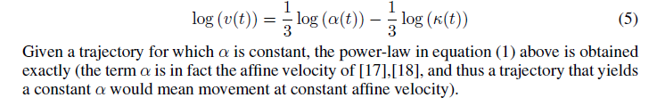
This is precisely the same mathematical relationship between curvature and velocity that we derived in the 2017 paper, but we used R for the measure of curvature rather than C so the coefficient of R was positive:
![]()
Maoz et al noted (under their equation above) that the 1/3 power law will be found when the affine velocity of the movement (alpha for Maoz, D for Marken & Shaffer) is constant, which is true. But it’s also true that the -1/3 power law will be found when affine velocity is variable but uncorrelated with variations in C. This is what we learn from the OVB (omitted variable bias) analysis that we describe in the 2017 paper.
Apparently, Maoz et al were looking at their equations as describing the physical relationship between variables, which is suggested by the fact that they add time indexes to the variables: v(t), kappa (t), alpha (t). But statistical regression analysis is used to determine whether a movement is power law conforming and regression analysis doesn’t care about the time at which the value of each variable was collected; it just cares that the values of each set of variables was collected at the same time.
So what this means is that you will find that curved movements conform to the -1/3 power law when 1) you use simple linear regression which 2) omits inclusion of the the affine velocity variable, D or K, and 3) cov(D, C)/var(C) is close to 0. This is why I call the finding of a -1/3 power law a side effect of control that results from a statistical artifact; it is a side effect that is seen when using a particular form of statistical regression analysis.
RSM
So, why didn’t you scientifically test the relationship between speed and curvature, to see if it is controlled or not? Instead, you only had a “realization” and claimed that it is a “side effect of control”.
By the way, why doesn’t “side effect of control” mean the same to you as “side effect of controlling something else”?
Strange use of language. There are many measures of behavior, no sense talk about “behavior itself”.
Did you really read it? Because it has nothing to do with R as a measure of curvature. I mean, try reading just the title.
I’m going to ingore the rest, as we’ve discussed it many times here. You can’t have something be a real effect found in movement, and simultaneously a statistical artifact.
My “realization” happened when I was asked by Alex how Bill’s model would explain the power law. So I thought about what I’m controlling when I move my finger around in different curved patterns. The most obvious controlled variable is the spatial position of the fingertip, which is being maintained in a varying reference state, protected from the effects of variable force disturbances.
So where would the speed-curvature power law come from? It couldn’t be a controlled variable because there is no way I could compensate for disturbances to, say, curvature, by varying speed, and vice versa. That’s because the outputs (muscle forces) that are moving the finger at a certain instantaneous speed are simultaneously moving the finger through a certain instantaneous curvature.
It was this “realization” that led me to suspect that the power law was simply a side effect of maintaining the position of the finger (or mouse or pointer) in a varying, curved reference state. And it’s this realization that then led me to notice that there might be a mathematical relationship between the calculated values of the variables involved in the power law.
So using all the high school algebra I could muster I found the following relationship between measures of speed (V) and curvature (R, which is the way curvature was measured before you showed that C = 1/R is a better measure to use):
V = R^1/3 * D^1/3
where D turns out to be a measure of affine velocity,
I was rather gobsmacked to see that there is, indeed, a mathematical 1/3 power relationship between speed (V) and curvature (R) for curved trajectories. This could certainly account for the 1/3 power law being a side effect of control of finger position in curved movements. But there was that pesky D term also. How would that affect the finding of a 1/3 power law? It turns out that how D affects the finding of a power law turns on how the power law is tested.
The 1/3 power law in curved movement is tested by regressing log C on log R; the regression equation that is tested is:
log V = k + beta1 (log R)
where beta1 is the power coefficient determined by the regression analysis. This analysis leaves out the variable D.
D can be included in the analysis using multiple regression, where the regression equation would then be:
log V = k + beta1 (log R) + beta2 (log D)
When you run this analysis on ANY curved movement you always find that k = 0, beta1 = 1/3, beta2 = 1/3 and R^2 = 1.0. This is because the regression analysis is picking up the fact that, for any curved movement the true relationship between V and R is the mathematical relationship V = R^1/3 * D^1/3.
Of course, this also holds when C rather than R is regressed on V since:
V = C^-1/3 * D^1/3
and the regression analysis will again always result in k = 0, beta1 = -1/3, beta2 = 1/3 and R^2 = 1.0 for any curved movement.
Leaving D out of the regression analysis affects the the value of beta1 – the power coefficient for curvature – and the size of R^2. The value of beta1 will deviate from its true value – 1/3 or -1/3 depending on whether R or C is used as the measure of curvature – by an amount proportional to the covariance of R (or C) with D. The size of this covariance term depends on characteristics of the curved movement that is produced and has nothing to do with how it’s produced. So the power relationship between speed and curvature that is found when D is omitted from the regression analysis depends completely on the nature of the curved movement that is produced and tells us nothing about how that movement was produced. It is in this sense that the power law is a statistical artifact; the power relationships between speed and curvature that have been observed are all a result of failing to include D in the regression analysis used evaluate that relationship. If D were included in these analysis then it would be come evident that the power coefficient relating curvature to speed is always exactly 1/3 (or -1/3) for all curved movements. It’s a mathematical law, not a law of behavior.
It does. It just doesn’t seem appropriate in this case because I quickly saw that the power law couldn’t possibly be a controlled variable, for reasons given above.
I imagine you will scorn all of this, if you read it at all. But I will say that I think your model of curved movement behavior has great promise and I’ll try to write a more positive review of it when I get the chance.
RSM
In PCT, there is a way to quantitatively test whether a proposed variable is controlled or not. This is called the test for the controlled variable. You should give it a try sometimes, instead of playing with algebra.
Here is another try to explan why:
What you see there are three variables, V, R and D. A relationship between three variables is very different from a relationship between two variables.
Take a set of rectangles of different sizes, width W, height H, and area A; random widths and heights. You can imagine them, but maybe best if you draw them out, or you can take an excel spreadsheet with a row for random widths, and random heights, and calculate their area in the third column.
For every rectangle in the set, there is a mathematical relationship between W, H and A. It is exactly A=W*H, or to make it a bit more similar to your formula, A= W^1 * H^1. Or we could write it as W = A * H^-1, or H = A * W^-1, or W = A/H, etc.
The relationship between these three variables is exact, always true, and yet there is absolutely no relationship between the width and the height of these rectangles - they are random. You can’t take the formula for the area of a rectangle to claim that widths are heghts are related, and that is exactly what you’re doing with the speed and curvature and affine velocity.
You’ve taken the formula for D to mean that speed and curvature are related. That is the mistake. The formula to calculate D is D =V^3 / R, or D = V^3 * R^-1. (You’re missing a minus somewhere in your formula).This is always an exact relatioship for every point in the trajectory, for any trajectory, and for any relationship between speed and curvature.
To continue the analogy with rectangles, the question of the speed-curvature power law would be like a phenomenon where all rectangles drawn by people were nearly square, and your claim would be - aha! I am gobsmacked! The area of each of those rectangles is A = W*H! There is a precise mathematical relationship between widths and heights in the the mathematics, and that is why everyone else thinks that people are drawing squares, because they are missing the variable A, the area. If you do multiple linear regression, you would see that the coefficients are exactly 1 and 1, not because the rectangles are squares, but because they are missing a predictor!
log W = b0 + b1 * log A - b2 * logH
omg! the b coefficietns are 0, 1 and 1, always! That is why people keep thinking widths are heights are related.
If it makes you feel any better, I’ve made a very similar mistake with angular speed, in my first paper on the power law. I write about it in that other paper I mentioned above. If angular speed is defined and A = VC, then A is going to be very trivially correlated to C, for any slightly larger range of C, even without V and C being correlated.
Adam, I appreciate your serious yet light-hearted style.
This post reminded me of Phil Runkel’s letter to Bill Powers of December 11, 1986, with Phil’s five-page dissertation on Traginology enclosed. See the Dialogue book, page 252 ff.
Keep up your good work!
What variable should I have tested for being for being a controlled variable?
My point exactly. Power law researchers have used regression to look only at the relationship between two variables, such as V and R. You often find a vary different relationship between these two variables when you include the third variable, D, as a predictor in the regression analysis.
But there is a probability that they will be correlated. The probability of seeing any particular correlation between two random variables is given by the probability distribution for the correlation coefficient, r, under the null hypothesis.
All of this reflects a remarkable lack of understanding of what I have shown. Your biggest mistake is assuming that multiple regression would find the correct coefficients for H and W (1 and 1) only if “all rectangles drawn by people were nearly square”. In fact, the correct coefficients would be found if H and W for each rectangle in the regression were set randomly.
I have demonstrated that this is the case in a little spreadsheet I created. When you regress H and W on A using the regression equation:
log (A) = betaH*log(H) + betaW *log (W)
where H and W for each rectangle are selected randomly the result is always betaH = 1.0, betaW = 1.0 and R^2 = 1.0
However, if you do a regression equation that leaves out one of the predictors, say W, so that the regression equation is:
log (A) = k + betaH*log(H)
then estimates of betaH, using different random sets of values for H and W, range from ~.7 to ~1.2 and the R^2 for the regression ranges from ~ 4 to ~.6.
The power law analysis is equivalent to regressing just H on A. The power law analysis, which uses just one of the variables to predict V, you get values for the coefficient that vary a bit around the actual value of the exponent (1 in the case of the rectangle, 1/3 in the case of the power law) but you will always get the exact value if you include both predictors.
Here’s a pointer to the spreadsheet, if anyone is interested. Just hit F9 to get new random values. Think of the regression of H on A as equivalent to what you are doing when you regress R (or C) on V.
RSM
I went and reread that now, very nice text!
Cheers!
You should have tested the relationship between speed and curvature. You keep saying that you had a realization that this relationship was a side-effect of control. And I keep saying that you should have tested that proposal using the TCV.
You can perceive curvature of the path. The letter U has low curvature on the sides, and high curvature on the lower part. You can perceive speed. You could, for example, move very slowly, at a constant speed, along the letter U. For very low speeds, you could even do this against slow disturbances.
It is perfectly possible to have a controlled variable be someting like “go slower in curves” relationship, just like in driving. The big question is what is the bandwidth of this ability, when do the disturbances become too difficult to control. At higher average speeds, we seem to loose this ability to intentionally control the speed-curvature relationship.
Oh, sigh… You have this pathological tendency to not admit you were wrong. I used to get so irritated by it. We discussed this point in particular so many times, but all of our discussions were are waste of time, because at some point in the discussion you would just start rambling rather than looking at the evidence, plots, experimetns, and seeing your mistakes. Why is it so difficult for you to see your mistakes?
No, if you include D in the multiple regression, you will get always the same result. The coefficients will always be 0, 1/3 and -1/3. It is an exact formula, you don’t need multiple regression. You don’t need statistics to discover that the area of a rectangle is width*height, just like you don’t need statistics to re-discover the formula for D.
I mean, sure. A bit irrelevant, but ok.
Oh, who are you quoting there? Multiple regression will always just return the coefficients from the formula, regardles of the W-H relationship, is what I said. It is really a completely useless procedure in this situation. Don’t ramble, concentrate. Do you want to come down to the “truth”, or do you just want to say shit until I give up?
Well, if you are using curvature and angular speed, then yes, it would be equivalent to correlating height and area. This should be avoided, because for a set of random rectangles of different sizes, rectangels of small height will tend to have small areas, and rectangles of large height will tend to have large areas. This correlation would not tell you much about the realtionship between widths and heights.
If you are correlating speed and curvature, then this is equivalent to correlating widths and heights, and is perfectly fine. Speed is independent of curvature, just like widths are independent of hegihts of rectangles. I don’t see it in your spreadsheet, but the W-H correlation should be near zero.
If you would want to find out if people draw squares, you could just correlate widths against heights. That is why most people correlate speed against curvature in their papers.
It is important that regression of H on A is not equivalent to R on V.
A s the equivalent to D, because we have formulas for them, A=WH, and D=V^3/R
By themselves, W and H are independent, and R an V are independent.
I don’t understand how one can test that. How did you disturb either of the variables, V or C, without disturbing the other? I think your model shows pretty clearly, as does mine that are described in Marken & Shaffer (2017), that the power law is a side effect of controlling another variable and is not itself a controlled variable.
So you believe that the speed-curvature relationship is a controlled variable, not a side-effect of control. Why do you think that this is the case? What “test” led you to determine that this is the case? Your model is not controlling for a power relationship between speed and curvature and yet it matches the subject data nearly perfectly, both when the subjects make movements consistent with the -1/3 power law (fast movement condition) and when they don’t (slow movement condition). It seems like the power law is just a side effect of controlling the position of the stylus, which is what your model ultimately controls.
Why is it so difficult for you to see yours?
I don’t use multiple regression to show that V = C^-1/3*D^1/3. I use it to show why regressing only C on V results in a power relationship with an exponent “close” to -1/3. It is only varies around -1/3 because you leave D out of the regression; include D and it is always exactly -1/3.
The size of the deviation from -1/3 depends on the covariance between C and the variable D, which is omitted from the regression; the closer the covariance of C with D, cov(C,D), is to zero the closer the observed coefficient of the speed-curvature relationship will be to the “power law” value of -1/3.
There are many ways for cov(C,D) to be close to zero. One way is for D to be nearly constant in a movement. Maov et al inferred this from the math. But there are other ways for cov(C,D) to be close to zero without D being constant. This means that the coefficient of the speed-curvature relationship that you find by regressing C on V, leaving out D, has nothing to do with how the movement was produced; it has only to do with the mathematical properties of the movement itself.
The observed power law relationship between speed and curvature in curved movement is, therefore, a side effect of controlling position (as in your model) and the appearance of this side effect as approximately a -1/3 power law is a side effect of regressing only C on V, omitting D. But it is a particularly seductive side effect because it looks like it shows that people making curved movements “slow down through curves”. But the apparent slowing down through curves is simply a result of the mathematical relationship between V and C, ignoring D: V = C^-1/3.
Actually, that is not only relevant, it’s the essential fact. The correlation (covariance) between C and D makes all the difference. When the correlation between C and D is low then the simple regression of C on V will result in a coefficient of C near -1/3 and an R^2 close to 1.0; when the correlation is high the coefficient of C will not be close to -1/3 and the R^2 will be low. And the correlation between C and D is a function of the nature of curved movement that is produced, not of how it was produced.
You.
Perhaps I misunderstood your misunderstanding. Here’s what you said:
This is all wrong. The proper analogy to what I am doing is this:
There is a bunch of high powered researchers who have been studying how people (and other organisms) produce rectangles of different sizes They have found that there is a consistent width-area power law that they think reveals something important about how rectangular movements are produced and they have been trying to explain the existence of this law for over a century.
These researchers measure the extent to which drawn rectangles follow the W-A power law by regressing log (W) on log (A), unaware that there is another variable, log (H), that contributes to the variance of log (A). The researchers have discovered that there is a pretty strong power relationship between log(W) and log (A) with a coefficient equal to 1.0 plus or minus .2. So they take this to be the W-A power law of rectangle drawing.
Then this guy who barely made it though junior high math comes along and points out that he has discovered that A actually depends on W and another variable, H by the formula A = W * H. So the true power coefficient of W is exactly 1.0. He claims that this can be proved by including log (H) in the regression on log (A), which always results in a regression solution with 1 as the coefficient of both W and H and an R^2 of 1.0.
This guy goes on to argue that this shows that the area - width power law is simply a consequence of the mathematical definition of A and has nothing to do with the mechanism by which people produce rectangles. For his troubles the guy who points this out is re-payed with score and contumely.
In your analogy, correlating width (W) and height (H) would be equivalent correlating curvature (C) and affine velocity (D). The analogy was:
V = C^-1/3 * D^1/3 for power “law” of movement
A = W^1 * H ^ 1 for the power law of rectangles.
I don’t think so but it doesn’t matter; I think the analogy is a good one.
I just put the W-H correlation into the spreadsheet. On repeated runs this correlation varies around the expected mean of the probability distribution which is 0.0 but it is often as high as .2 or -.2 but it can occasionally go even higher. Since C and D are not completely independent the expected mean of the probability distribution of correlations seems to be around .25 and often goes as high as .45. The correlation never goes negative so I assume the probability distribution of the correlation is similar to the Poisson.
This is simply not true. It is precisely equivalent.
But that equivalence has nothing to do with how the regression is carried out.
Again, the analogy you proposed is this:
A = W^1 * H ^ 1 is analogous to
V = C^-1/3 * D^1/3
and these equations are linearized for regression by taking the log of both sides so:
log (A) = 1*log (W) + 1 * log (H)
log (V) = -1/3* log (C) + 1/3 * log (D)
The power law is determined by regressing log (C) on log (V). This is analogous to regressing log (W) on log (A).
The regression analysis doesn’t care how any of the variables were calculated; they are just numbers that go into the regression machine. But the results of this simple regression depend on how the variable included in the regression correlates with the variable left out.
RSM
V and C are independent variables, you can disturb them independently. For example, you can have the same shape traversed with different speed profiles, or you can have the different shapes traversed with same speed profiles, etc. Each of those situations can have a different relationship between speed and curvature.
For example, in experiment #1 in this paper, the target always moves along an ellipse, and the speed profile is changed to follow a different power law.
You can see this as a form of TCV. For slow rhythms, participants CAN follow the targets allong different speed profiles. The speed of the cursor is very close to the speed of the targets. This does not show that the speed-curvature power law is a controlled variable (it could be), but it does show that at low average speed, regardless of the curvature, the participants can control their instantaneous speed.
The more interesting case are fast targets - here the particants cannot follow different speed profiles of the target, so the power law relationship is not a controlled variable, and is probably a side-effect of controlling something else.
Mine does, but your does not show. You only claim that, but don’t do any TCVs.
Please, let’s stick to this one. So, the slowing down in curves is only apparent?
Would you agree that this claim is wrong if I show you empirical data that slowing down is real?
They claim that the WIDTH-HEIGHT power law is important and also equivalent to the widith-area power law.
You claim that both the width-height power law, and the width-area power law are statistical artifacts, but they are not. There is a problem with the width-area power law that shows higher correlations, but the width-height power law is fine.
No, the analogy I proposed is:
D = V^3 * R^-1
A = W * H
I’m proposing that the width and height are analogous to speed and curvature, because you can change the width of a rectangle without changing the height. The area of a rectangle cannot be changed without changing either width or height, just like D depends on curvature and speed - you can’t calculate D without knowing V and C. But you can find V without knowing C and D, and you can find C without knowing V and D.
The important part is that we are looking for the relationship between width and height, not between area and width.
In the spreadsheet, for random W and H, the correlation between them will be low, as you say (if you put more samples, it will not go near .2). And this is simply showing the true and important relationship that we are looking for. Are the people drawing squares? In this case, no, widths and heights are random, and the simple W-H correlation gives the expected result.
The W-A correlation can be high, as I’ve mentionied, because of the range of widths. If you make the range of W bigger, while W still being random, the W-A correlation can grow up to 1, without the rectangles being any more square. This just means that small-W rectangles have small areas, and big-W rectangles have a big area.
But, again, let’s stick to your claim that the slowing down in curves is only apparent. How can you claim this if the empirical data shows slowing down in curves? And more importantly - what would change your oppinion, what kind of evidence?