Visuomotor phase-locked loop reproduces elliptic hand trajectories across different rhythms [preprint]

RM: Temperature is probably only one of the variables that affects that relationship. There are surely others as well, such as seasonal variations in vacation taking and school attendance.

Surely, but that does not weaken the fact that there is (or at least can be) a causal (physical) dependency between some (at the moment more or less unknown) physical causes and both ice cream sales and murder rates. This kind of causal dependency can then cause the statistical correlation between ice cream sales and murder rates. That latter correlation between ice cream sales and murder rates is not a statistical artefact even though there were no causal relationships between them.

RM: The relationship is observed by a researcher who fails (surely unintentionally) to include all the possible predictors of yearly variations in murder rate into their prediction equation.

Yes, surely fails, but that does not make the dependency a statistical artefact. It makes it only a less than perfectly understood causal / physical relationship – not between ice cream sales and murder rates but between them and some other factors.

RM: What relationship are you talking about? All we’ve observed is a correlation between ice cream sales and murder rate. Temperature is one likely covariate that could account for the existence of this relationship. What do you think is a physical artifact?

I suggest to call the correlation between ice cream sales and murder rate a physical artefact (probably not best possible name) because that correlation does NOT depict a causal relationship between these two variables but instead is caused causally / physically by (at the moment unknown) third group of variables. That correlation is not created statistically by the observer but physically by some unknown influencers like temperature etc.

EP (earlier): Instead if you calculate a dependency between curvature and speed by using their common cross product as an extra predictor, that is really a statistical artefact.

RM: No, actually it’s called multivariate analysis or analysis of covariance (ANCOVA).

What I hope you should understand is that the affine speed is a variable which can be calculated from the speed and curvature. It is not an independent physical variable which could and should be added to multivariate analysis. It is as dependent from speed and curvature as the area is dependent on height and width of a quadrangle. Or as bachelorhood is dependent on malehood and nonmarriage. If you add these kind of doubled extra predictors then it creates a statistical artefact.

Yes, excellent observation. Affine velocity (A) can, indeed, be calculated from speed (V) and curvature (C), just as V can be calculated from C and A and C can be calculated from A and V. This is because all these variables are mathematically related and any one of them could be considered a dependent variable as a function of the others as independent variables.

Since regression analysis is used to evaluate these relationships it’s probably better to use the terms criterion variable and predictor variables to refer to the variables in the roles of dependent variable and independent variables, respectively.

Here are the equations for each of the variables V, A and C in the role of criterion variable, linearized for regression analysis. First the familiar equation with log V as the criterion and log C and log A as the predictor variables:

log V = -1/3 * log C + 1/3 * log A (1)

Next the equation with log A as the criterion variable and log C and log V as the predictors:

log A = log C + 3 * log V (2)

And finally with log C as the criterion variable an log V and log A as the predictors:

log C = - 3 * log V + log A (3)

Power law researchers have been obsessed with studying the relationship between C and V with V as the criterion and C as the predictor variable. They study the relationship using the following regression equation:

log V = k + beta * log C (4)

This equation is only part of the actual mathematical relationship between log V and log C, as shown in equation (1). What’s missing is the affine velocity predictor variable, log A. This means that the solution of the regression will depend on the degree to which the included predictor (log C) is correlated with the omitted one (log A) in that particular movement.

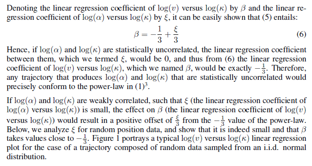
Per equation (1), the true (mathematical) value of beta in (4) is -1/3. But with log A omitted from the analysis, the regression will find the value of beta to deviate from the true value by an amount the is proportional the covariance between log C and log A.

The same would be true if researchers were interested in studying the relationship between C and A with A as the criterion variable and C as the predictor.

log A = k + beta * log C (5)

In this case the true beta, per equation (2), is 1.0. But the beta value found by the regression analysis will deviate from 1.0 by an amount that depends on the covariance between the included predictor, log C, and the omitted predictor, log V.

And, of course, the same would be true if the researchers were studying the relationship between C and V, with C as the criterion variable and V as the predictor. In that case the repression equation would be:

log C = k + beta * log V (6)

Now the true beta, per equation (3), is 3.0. But, again, the beta value found by the regression analysis will deviate from 3.0 by an amount that depends on the covariance between the included predictor, log V, and the omitted predictor, log A.

What all of this shows is that there is, indeed, a mathematical relationship between the variables V, C and A. When you study the relationship between any two of these variables using regression analysis, the result will be an estimate of the coefficient of the predictor variable that deviates from its true, mathematical value to the extent that the third, omitted variable, covaries with that predictor; the higher the covariation, the greater the deviation from the true value.

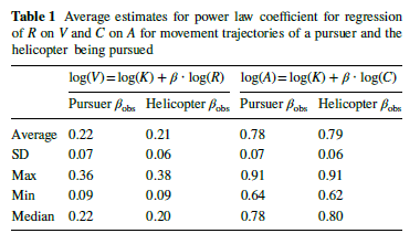
Maob et al have found that, when using only two of the three variables (V and C) in a regression analysis, the deviation from the true value of the coefficient relating the two is typically quite small. They suggest that this is because the deviation from the true value is proportional to the covariance between the two divided by three. So the covariance has to be quite large for the deviation of observed from true beta to be large.

When regressing C on V (equation 4) the true (mathematical) value of the coefficient relating C to V, -1/3, corresponds to what has been called the “power law” or "-1/3 power law. Maob et al have shown that the best way to find this law (that is, the best way to get -1/3 as the value of beta from this regression) is to low pass filter the observed movement data. Apparently such filtering reduces the covariation between the included (log C) and omitted (log A) predictor variables.

Thus, the finding of a power law relationship between two variables, such as between V and C, is an artifact in the sense that it is “something observed in a scientific investigation or experiment that is not naturally present but occurs as a result of the preparative or investigative procedure”; filtering being being the preparative procedure. But I would also say it is a statistical artifact since, per the Oxford dictionary, “a statistical artefact is an inference that results from bias in the collection or manipulation of data”; filtering being a way to manipulate the data.

I think the power law – the one that views V as a -1/3 power function of C – has become the focus of a lot of research on movement production because it seems to make intuitive sense: it suggests that when producing curved movement organisms “slow down through curves”, just as a driver would do when going through curves. But it’s also possible to look at it the other way around, with log C as the criterion and log V the predictor, per equation (6). And what we would see is a power relation with a coefficient close to -3 suggesting that organisms “widen curves when they speed up”, which is also something drivers do; they cut corners when they are going faster.

Both views are consistent with the data. But both views are illusions in the sense that they don’t reflect what the organism is doing (controlling); they are a side effect of the mathematical relationship that exists between C, V and A, combined with the filtering of the data that is being analyzed.

“Both views are consistent with the data. But both views are illusions in the sense that they don’t reflect what the organism is doing (controlling)”
Shouldn’t that sentence end with the specific perceptual variable(s) being controlled? Surely, the judgment of whether the power law is a statistical artefact can only be made with respect to a certain theory of control (e.g. PCT) and a certain variable(s), and even a certain gain, delay, reference value of that variable(s)?

The point of my post was that the “power law” of movement can be found regardless of how the movement is produced. We actually showed this in Table 1 of [Marken & Shaffer (2017)](file:///C:/Users/Rick%20Marken/Dropbox/MarkenShaffer2017.pdf), copied below:

image

The Table shows the power coefficients for curved ground trace movements made by people pursuing toy helicopters (Pursuers) and by the helicopters themselves (Helicopter). Note that the average power (beta) coefficients for movements made by Pursuers and Helicopters are about the same. These averages are somewhat lower than the 1/3 power law but they are consistent with what is found in much of the power law literature. And you can see from the max values that the power coefficient can be closer to .33 on many occasions.

This result shows that you will get something close to a power law from movements produced by a control system – a system that is controlling some perceptual variable – and from a purely causal system – which is not controlling anything. Once you know that velocity, curvature and affine velocity are mathematically related to one another by a power relationship and that the power law is determined by including only two of these three variables, curvature and velocity, which have a power relationship of 1/3 (or -1/3 if you are measuring curvature as 1/R) in a regression analysis, you know that the regression analysis will produce the same results and results that are close to 1/3, whether the movement is produced by a control system or a causal system.

So, no, you don’t need to know what variables the system making the movements controls or even whether it is a control system making the movements in order to know that the power law is a statistical artifact.

Wow. So there are no conditions, parameter combinations or specific controlled variables for which the power law doesn’t emerge?

Rick completely mis-states the point of at least my criticism of his Power Law paper. It was simply a high-school level mathematical error in his reasoning that completely invalidated his analysis. When a tautology is fit by an infinity of (all possible) values, a claim must be challenged that its fit by a particular value is evidence for something important. That he still believes his mathematics was correct indicates that his control for having been correct wins a conflict with any control he may have of a perception that his work is mathematically supportable. Or that he never took algebra in early high school.

A model that accurately mimics the behavior (controlling) being modeled will produce the same side effects as that behavior. Adam demonstrated this with his two level model of curved movement. The model accurately mimics the human controlling in both the slow and fast movement conditions. But the -1/3 power law side effect is only seen in the behavior of the model in the fast condition, as was the case for the behavior of the human.

Bill’s CT psychology is aimed at understanding control, not the side effects thereof. Once you have a good model of an example of controlling – like Adam’s model of tracking – then the side effects of that controlling will automatically “fall out” of the model; the side effects will be seen when the model behaves in the same circumstances as the behaving system being modeled.

So the “parameter combinations or specific controlled variables for which the power law doesn’t emerge” are the same as the ones for which it does emerge; they are the ones that give the best fit to behavior (in this case the behavior of producing curved movement). Trying to produce a model that mimics some side effect of behavior is just a sideways (and rather inefficient) approach to developing a model of the behavior itself.

Since my mathematical analysis of the power law was exactly the same as that of Maob et al, your criticism of my math applies to theirs as well.

We both found that:

log V = 1/3 log R + 1/3 log D (1)

where V is velocity, R is radius of curvature and D is affine velocity. (Actually, Maob et al used curvature, C, as the measure of curvature and since C = 1/R their first term on the right was -1/3 log C).

After some eye-crossing math, you ended up proving that equation (1) is a big mistake because it is just a tautology:

log V = log V

This is something that could have been shown without all the complicated math. Since the right side of (1) = log V then we can substitute log V for 1/3 log R + 1/3 log D and re-write equation (1) as:

log V = log V.

QED.

I suppose this is a tautology but, when unpacked, so to speak, as equation (1), it leads to very interesting insights about why something close to the 1/3 power law is typically found as a side effect of making curved movements.

I guess the one who said it best might have been Admiral Nelson, who, at the battle of Trafalgar was told that the senior Admiral had hoisted a signal. On which he put his telescope to his blind eye and said “I see no signal” and went ahead to execute his battle plan.

It’s OK, Rick, you can carry on however you want, putting your “mathematical telescope” to your mathematical blind eye. Maybe bulling ahead as Nelson did won’t win you the battle, if there ever was a battle, but I suppose it will gain you some non-mathematical believer fans, which I suppose is something for which you control.

There is none so blind as he who will not see.

I’d be interested in your evaluation of the Maob et al analysis.

”excellent observation” ??? How many times it has been told and shown you in this discussion. Good that you now agree to see that all these:

log V = -1/3 * log C + 1/3 * log A (1)

log A = log C + 3 * log V (2)

log C = - 3 * log V + log A (3)

are tautologies. Actually they are definitions (or forms of the same definition) of the affine velocity A. There are only two independently varying variables V and C which have no mathematical relationships between them. Then there is a fully (mathematically) dependent variable A which is defined by the two other variables.

Just like in the Adams earlier good example the about the width (w), height (h) and area (a) of a rectangle. The area is defined and fully (mathematically) dependent on the two other variables height and width; while width and height are totally (mathematically) independent from each other:

a = h * w

h = a / w

w = a / h

Can you see the identity between these two cases? They are even structurally identical with the definition:

bachelor = unmarried male

These kind of definitions are useful to introduce new concepts, and bachelor, area of a rectangle and even affine velocity are handy concepts for some needs. Why affine velocity is defined and in that complicated way with those 1/3 multipliers? Probably because it is in some situations a useful way to express that a trajectory obeys 1/3 power law by saying that the affine velocity is stable. These expression mean the same!

I took a look at that Maob et al. They note passing that “the term α is in fact the affine velocity of [17],[18], and thus a trajectory that yields a constant α would mean movement at constant affine velocity” but I can’t find them making such fancy claims like you that there is some mathematical dependency between speed and curvature and that this dependency should be unveiled by adding affine velocity as a predictor to the multivariate correlation analysis. That procedure will only show the tautological correlation between the defined and defining variables. Instead they claim that power law phenomenon has much to do with noise. Both with noise in the production of the movement and in the measurement of the movement. Unlike you they admit that “We do not suggest that the power-law, which stems from analysis of human data, is a bogus phenomenon”.

Rick,

Your diversion from your own mistake to asking me to check someone else’s maths is, from you, “classical”. The only issue is that in your paper you use logic of this form.
Aristotle is a man.
I see a man over there.
I’ve always wanted to talk to Aristotle.
So I must go over and talk to him now.

Martin

I don’t agree that they are tautologies; I think they are mathematical expressions of the relationship between three variables, velocity (V), curvature (C) and affine velocity (A). Equation(1) is the most relevant because it describes the mathematical relationship between log C and log V when log V is the criterion variable and log C the predictor. It shows that the true mathematical relationship between log V and log C includes the variable log A. This is precisely what was shown by Maob et in their equation (5)
image
where their v(t) is equivalent to V, their alpha (t) is equivalent to A and their kappa(t) is equivalent to C in equation (1) above.

Perhaps you didn’t notice but they make the same “fancy” claims as I do right here:
image

Their equation (6) is equivalent to our OVB (omitted variable bias) analysis. It says that the observed power law coefficient found when regressing log C on log V, omitting log A, will deviate from its mathematical value (-1/3 as shown in equation (1) above) by an amount proportional to the covariance, eta, (measured as the regression coefficient) between log A and log C. If that correlation is zero then the observed beta will be exactly equal to the mathematical value of beta, -1/3.

I think it’s understandable that they would “admit” that, despite the obvious implications of their analysis. They are prominent power law researchers talking to an audience of other prominent power law researchers.

This is a good example of why Powers’ brilliant work has had such a hard time being understood and/or accepted by “mainstream” behavioral researchers and neuroscientists. That’s why I find it amazing that his 1978 Psych Review paper was published in a prominent psychology journal. In that article he implicitly says what he said explicitly in his Foreword to my book MIND READINGS" “Nearly every model in these pages, which did make it past the referees, is the sort that ought to convey to the reader a straightforward message: if the phenomenon you see here works as this model shows it to work, then a whole segment of the scientific literature needs to be deposited in the wastebasket.”

In our papers on the power law we never said it was a bogus phenomenon. It’s a real phenomenon. We were just saying that the phenomenon is a side effect of control and is observed because of the mathematical relationship between curvature and velocity (equation (1) above and Maob et al’s equation (5) ) and the way the relationship between these variables is analyzed.

It wasn’t meant as a diversion but, rather, an opportunity for you to explain what my mistake was in terms of what Maob’s mistake wasn’t. I’m assuming that Maob et al didn’t make a mistake because their paper was referenced approvingly in the critical reply to our paper. But if you could show me that they did make a mistake that would be very informative also since it looks to me like their mathematical analysis is identical to mine.

Ok, perhaps definition is a better word here than tautology (even though every definition and identity equation is a tautology). But I asked also can you see the (structural) identity between the definitions of affine velocity, area and bachelor? If not, what is the difference (in addition to those that area is simpler that affine velocity and bachelor is not mathematically defined)?

The affine velocity is defined in Pollick & Sapiro 1996. Their process of derivation and reasoning is quite complicated but the idea and result is simple: They produced a mathematical concept, a variable called affine velocity which behaves so that if (and where) a movement obeys 1/3 power law then the affine velocity of that movement remains stable. They also tested this empirically and from that becomes their title “Constant Affine Velocity Predicts the 1/3 Power Law…” which is a little misleading because constant affine velocity does not only predict but it means the same as 1/3 Power Law (if affine velocity is defined in the way they did it).

Compare this behavior to that of an area of a rectangle: a = w * h. If you have a sample of different rectangles and you find out that their a is always same – it remains stable of constant - then you can infer that their w and h must have full negative correlation between them, mustn’t they? This is exactly similar situation than with affine velocity and power law except that the powers and multipliers in the definitions are different.

As you say those definitions 1,2,3 are of course mathematical expression but not strictly speaking of the relationship between three variables, because they can say nothing about the relationship between velocity and curvature - as well as the definition of the area can say nothing about the relationship between width and height - because their relationships are purely empirical, there is no mathematical relationship. Instead these definitions express the mathematical relationship between affine velocity in one hand and both velocity and curvature in the other hand because they define affine velocity in relation to velocity and curvature. (just like a = w * h defines area in relation to width and height of a rectangle.)

Yes, Maoz et al said: “if log(α) and log(κ) are statistically uncorrelated, the linear regression coefficient between them, which we termed ξ, would be 0, and thus from (6) the linear regression coefficient of log(v) versus log(κ), which we named β, would be exactly −1/3.” For me this means that if affine velocity and curvature are uncorrelated – which happens if affine velocity is constant – then there is -1/3 correlation coefficient between velocity and curvature, which means that the movement obeys 1/3 power law. This follows from the definition of the affine velocity. Nothing else follows from this and Maoz et al seem not to claim anything else.

The definition of affine velocity thus has two components, curvature and normal or Euclidean velocity. If you use this construct as an extra predictor in a multivariate correlation analysis between curvature and velocity it means that there will be curvature twice and velocity in the both sides. So you will analyze the correlation of velocity to itself. Because the definition of affine velocity is originally tweaked to fit with 1/3 power law then it should be no surprise that you will get 1/3 correlation coefficient even when there is absolutely no correlation between curvature and velocity as in cases where velocity is constant or the trajectory is straight line. That correlation result IS a bogus phenomenon.

RM: We were just saying that the phenomenon [power law] is a side effect of control and is observed because of the mathematical relationship between curvature and velocity (equation (1) above and Maob et al’s equation (5) ) and the way the relationship between these variables is analyzed.

Here you should decide what you want to claim:

  1. If you say that power law follows from the mathematical relationship between velocity and curvature then you will be ridiculed, because no sober researcher would believe that there is such necessary relationship between these two clearly both conceptually and empirically independent variables.
  2. Or if you say that the phenomenon is a statistical artifact (= bocus phenomenon!) produced by the arbitrary methods of the researchers (one good example of that is your OVB) then it cannot be a side effect of the control of the moving subject.
  3. Or if you want to say that it is a side effect of a control of a moving subject then you should show how the outputs of that controlling system produce that phenomenon as a side effect of it’s control. If you cannot show this then you have no reasons for that claim.
  4. Perhaps best is to admit that we do not yet know.

Best
Eetu

I said something a bit more nuanced than that the power law follows from the mathematical relationship between velocity and curvature. Nevertheless, I did get ridiculed for saying it.

I never said – nor do I think – that the methods used by the researchers are arbitrary. They are perfectly reasonable under the assumption that movement production is an open-loop process. However, once you understand that movement production is a control process then you know that the power law must be a side effect of this controlling. The statistical analysis (done by Maob et al and Marken & Shaffer) just shows why this side effect tends to be close to a 1/3 power “law”.

Adam’s model (and ours) has already shown how the outputs of a movement control system can produce (and not produce) the power law as a side effect.

I disagree. One of the most important implications of Powers’ model of behavior is that, as Bill put it in the Foreword to MIND READINGS “… a whole segment of the scientific literature [in the behavioral sciences] needs to be deposited in the wastebasket.” It is the segment that has been dedicated to the study of things that are actually irrelevant side effects of control, things like operant conditioning, circumstance X causes behavior Y, etc.

I think it’s pretty clear that the power law is one of those scientific findings that Powers’ model says should be deposited in the wastebasket – or at least ignored. Yet, to my considerable surprise, this has been a minority (of one) opinion here in this discussion group. I would like to know why. What does the power law have to do with PCT? If, as has been claimed, we all agree that it is a side effect of control, then why keep studying it? Why not just study how movement is produced? What variables are being controlled? How these control processes are organized?

Rick,

So you do it again and quite calmly dismiss the criticism which explains why your argument does not hold. It shows that you do not care about the validity of your argumentation and that is by definition the case of argumentative bs (Mukerji & Mannino 2022).

RM: I said something a bit more nuanced than that the power law follows from the mathematical relationship between velocity and curvature. Nevertheless, I did get ridiculed for saying it.

No wonder! I wonder why the article get published at all, but the academic filters leak as we know. The core of you claim was that there is a necessary mathematical relationship between velocity and curvature and the “true” correlation coefficient between them is exactly 1/3. It is actually just the same it you would claim that there is a mathematical relationship between the width and height of a rectangle and true correlation coefficient between them is 1. (i.e. all rectangles are in reality squares even if their width and height does not seem same.)

RM: I never said – nor do I think – that the methods used by the researchers are arbitrary. They are perfectly reasonable under the assumption that movement production is an open-loop process. However, once you understand that movement production is a control process then you know that the power law must be a side effect of this controlling. The statistical analysis (done by Maob et al and Marken & Shaffer) just shows why this side effect tends to be close to a 1/3 power “law”.

You have said that power law is a statistical artifact and that means that it is produced as a result of methods which do not fit to reality – which are arbitrary. From the fact that movement production is a control process dos no way necessarily follow that power law is a side effect of that controlling. It is probable but not necessary. Do not blame Maoz et al, they do not make such problematic inferences as you did. Your analysis only shows that if you use your very arbitrary and against the rules method of adding the velocity and curvature twice to the correlation analysis then you get always close to 1/3 correlation.

I don’t recall doing that intentionally. Perhaps what you are seeing is a side effect of my failure to see any criticism in your posts that explains why my argument does not hold.

Again, you are coming to conclusions about my intentions (what I care about) based only on my overt behavior. Actually, I care very much about the validity of my arguments and I am willing to change my mind if I am shown that my arguments are incorrect.

Actually, that paper was accepted for publication faster than almost any paper I’ve written, and in a journal where much of the power law research has been published.

No wonder you think my argument is BS. Your description of my “claim” is almost completely incorrect.

I do “claim”, as did Maoz et al, that there is a mathematical relationship between velocity (V) and curvature (C), the linear version of which is as follows:

log V = - 1/3* log C + 1/3 * log A

where A is affine velocity. In this equation -1/3 is the true coefficient of the power relationship between C and V, NOT the true correlation.

What this equation shows is that when you do a regression between log C and log V to determine the coefficient of the power relationship between C and V, using the regression equation:

log V = log k + beta* log C

you are leaving out one of the variables, A, that is involved in the mathematical relationship between C and V.

What Moaz et al and Marken & Shaffer (2017) showed is that when you leave variable A out of the regression equation, the observed value of the coefficient, beta, will differ from its true value, -1/3, by an amount proportional to the covariance between log C and the omitted variable, log A. This covariance will be different for different movement patterns but, as Maoz et al note, it will generally be small. So in a simple regression where C is regressed on V, the observed value of beta will generally not differ much from -1/3.

This analysis is not at all the same as if we had claimed that “there is a mathematical relationship between the width and height of a rectangle”. The proper analogy is this:
Using simple regression analysis of the form:

log A = log k + beta * log H

where A is area and H is height, researchers have found that A is a linear function of H sine beta will be approximately 1. The Maoz et al come along and point out that there is a mathematical relationship between A and H that includes another variable, W (width), so that the true relationship between log A and log H is

log A = log H + log W

So the true coefficient of H is 1.0 exactly and it is only approximately 1.0 when log W is left out of the regression analysis. This is because the beta calculated for log H depends on the covariance of log H and the omitted variable, log W.

The choice of analysis methods has nothing to do with whether they fit reality. Rather, they are chosen as the means of getting results that are presumed to give the best reflection of what constitutes the reality on the other side of our senses. The results of the use a particular analysis are artefactual if those results were “forced” by the way the data was collected or selected for analysis. The power law is a statistical artifact because the data is included in the analysis only after filtering and only a subset (V, C) of the variables (V, C, and A) that are known to be mathematically related are included in the analysis.

I didn’t blame Maoz et al for anything. I praised their analysis.

OK, it looks like that’s your story and your stickin’ to it. But I would like to know where you think the power law fits into PCT. You know where I think it fits: It’s an example of an irrelevant side effect of controlling. Where do you think it fits in?

RM: I don’t recall doing that intentionally. Perhaps what you are seeing is a side effect of my failure to see any criticism in your posts that explains why my argument does not hold.

So you accidentally did not read my whole message and jumped to comment only the end reflections. But yes, so it must be that you control for not seeing criticism and faults in your work, to perceive that you are right, and as a side effect produce omissions and that the name of which should not be said.

RM: Actually, I care very much about the validity of my arguments and I am willing to change my mind if I am shown that my arguments are incorrect.

It is seemingly impossible to show something to someone if that someone controls for not seeing that something.

EP (earlier): The core of you claim was that there is a necessary mathematical relationship between velocity and curvature and the “true” correlation coefficient between them is exactly 1/3. It is actually just the same it you would claim that there is a mathematical relationship between the width and height of a rectangle and true correlation coefficient between them is 1. (i.e. all rectangles are in reality squares even if their width and height does not seem same.)

Sorry, I mixed here the terms correlation coefficient and power coefficient, but that does not affect the criticism.

RM: I do “claim”, as did Maoz et al, that there is a mathematical relationship between velocity (V) and curvature (C), the linear version of which is as follows:
log V = - 1/3* log C + 1/3 * log A
where A is affine velocity. In this equation -1/3 is the true coefficient of the power relationship between C and V, NOT the true correlation.

No, Maoz et al do not claim this. They play a lot with affine velocity but they do not claim that there is any mathematical relationship between (Euclidian) velocity and curvature. Those equations (containing V, C, and A) are valid because they are just forms of the definitions of affine velocity. And if in trajectory the affine velocity remains stable then the power coefficient is 1/3. (If A is not constant then coefficient can be what ever if there is any.)

RM: What this equation shows is that when you do a regression between log C and log V to determine the coefficient of the power relationship between C and V, using the regression equation:
log V = log k + beta* log C
you are leaving out one of the variables, A, that is involved in the mathematical relationship between C and V.

You just keep repeating this and refuse to see that the definition of affine velocity cannot create any mathematical relationship between C and V. No more than the definition of the area of a rectangle could create a mathematical relationship between width and height of a rectangle.

RM: What Moaz et al and Marken & Shaffer (2017) showed is that when you leave variable A out of the regressino the observed value of the coefficient, beta, will differ from the true value of the coefficient, -1/3/ by an amount proportional to the covariance between log C and the omitted variable, log A. This covariance will be different for different movement patterns but, as Maoz et al note, it will generally by small. So in a simple regression where C is regressed on V, the observed value of beta will generally be close to -1/3.

This all will follow from the way how affine velocity is defined. I will no more try to evaluate the soundness of Maoz et al but you clearly make inferences what they do not make.

RM: This analysis is not at all the same as if we had claimed that “there is a mathematical relationship between the width and height of a rectangle”. The proper analogy is this: Using simple regression analysis of the form:
log A = log k + beta * log H [is log k accidentally here?]
where A is area and H is height, researchers have found that A \ is a power function of H with an exponent of approximately 1. Someone points out that there is a mathematical relationship between A and H that includes another variable, W (width), and the true relationship between log A and log H is
log A = log H + log W
So the true coefficient of H is 1.0 exactly and it is only approximately 1.0 when log W is left out of the regression analysis. This is because the beta calculated for log H depends on the covariance of log H and the omitted variable, log W.

Here you really don’t see the structural similarity between definitions of (rectangular) area and affine velocity, do you? Width and height are simple independent variables which can be measures as such. So are velocity and curvature of a trajectory. You can measure plain velocity and plain curvature. But when you want to determine the area of a rectangle, the basic and natural method is to calculate it from width and height. (Actually I cannot imagine a way to measure an area of a rectangle which would not reduce back to calculating in it from width and height.) Similarly you cannot determine affine velocity in another way than calculating it from velocity and curvature.

In power law research they are interested in the relationship between the independently changing variables velocity and curvature. The construction of the third variable, affine velocity whose value depends on the values of velocity and curvature, does not change this any way. It only brings to light a special case of trajectories where that affine velocity is constant, and in exactly this case the trajectory obeys 1/3 power law.

So the analogy must start from found empirical relationships between width and height of rectangles. In some cases there is this relationship and in some other cases another, but often they correlate strongly. (And unlike velocity and curvature positively.) Now someone defines a new variable, area, in this way: A = W * H. They also note that if A remains constant then there is a strong negative dependency between W and H. (Just like with affine velocity.) We can stop the analogy here but it should be clear that area does not create any mathematical relationship between width and height – they vary as independently as ever. And similarly affine velocity does not create mathematical relationship between velocity and curvature. But area can tell you that IF it remains constant THEN there is -1 correlation between width and height. And affine velocity can tell that IF it remains constant THEN there is 1/3 power law relationship between velocity and curvature, no more.

RM: OK, it looks like that’s your story and your stickin’ to it. But I would like to know where you think the power law fits into PCT. You know where I think it fits in: It’s an example of an irrelevant side effect of controlling. Where do you think it fits in?

In this kind of discussion group we should not be so much interested about what is whose story but what story is true and valid when compared together. The most tragicomic feature in your story (and consequently my criticism of it) is that it has nothing at all to do with PCT except that the fame of PCT as a serious scientific truth seeking enterprise is put under danger. Yes I know that you claim that power law is a side effect of controlling. And we know that so think all the other discussers here. At least it is the most probable alternative. But it has nothing to do with your mathematical reasoning which I and others have criticized. And as I have said, side effects are often interesting and important research topics.

Best,

Eetu

One thing I am specifically controlling for in this discussion is convincing you that the mathematical analyses of the power law by Maoz et al (2005) and by Marken & Shaffer (2017) are identical. You are trying to convince me that they are different and, moreover, that our analysis is mathematically wrong.

In an earlier post I explained this equivalence. None of your replies have directly addressed this explanation. So I will explain it again and see if you can tell me what is different about the analyses, with special emphasis on why theirs is right and ours is wrong.

Both Marken & Shaffer (M&S) and Maoz et al (Maoz) start with the observation that:

log V = 1/3 * log A - 1/3* log C …(1)

where V = velocity, A = affine velocity and C = curvature

The only difference between the M&S and Maoz equations is the symbols used for V, A and C.

Equation (1) describes the mathematical relationship between log V, log A and log C when log V is considered the dependent variable and log A and log C are the independent variables. The relationship between these variables is written this way because log V is always the dependent variable and log C the independent variable when regression analysis is used to test whether a particular movement conforms to the power law.

In power law tests there is only one independent variable used in the analysis, log C. So the regression equation used to test for a power law is:

log V = log k + beta * log C …(2)

where beta is the unknown power coefficient. The regression analysis is done by calculating log V and log C from the x,y coordinates of a filtered movement. If the movement lasted 100 secs and its x,y coordinates were sampled at a rate of 10 sample/sec, then you will have 1000 x,y values but only 998 measures of log V, log A and log C because the calculation of A and C involves calculating second derivatives.

The regression analysis based on equation (2) solves for values of beta and log k that gives the best fit (least squares criterion) to the relationship between log C and log V. For most curved movements, the beta that gives the best fit to the data is -.33 plus or minus .1 and the R^2 measure of goodness of fit is typically greater than .75.

Most of this regressing of log C on log V to test the power law was done for years before anyone thought to see if there is a mathematical relationship between log V and log C. But finally, for different reasons, Maoz (in 2005) and M&S (in 2017) did find that there is a mathematical relationship between these variables – the relationship shown in equation (1); it is a power relationship with a coefficient of -1/3 (or 1/3 if you measure curvature as R).

So the mathematical relationship between log C and log V is very close to what researchers thought was a behavioral law – the 1/3 power law. This must have been a very disturbing realization. But it seemed like there might be a way out of the obvious implications of this embarrassing discovery.

The relationship between log C and log V involves a third variable, log A. Maoz and M&S realized that this means that the results of a regression of log C on log V, sans log A, will result in an estimate of beta – the power coefficient – that might deviate from its mathematical value, -1/3. And both Maoz and M&S derived exactly how much beta would deviate from -1/3 when log A is omitted from the regression.

According to Maoz the observed beta would deviate from -1/3 by an amount proportional to the covariance between log C and log A. Their equation for this deviation is:

image…(3)
where
image…(4)

where their kappa is equivalent to C and their alpha is equivalent to A.

What equation (3) says is that the beta you will observe in a regression of just log C on log V will be equal to its true mathematical value, -1/3, plus a deviation term, eta/3. Eta is the regression coefficient for predicting log C from log A and, per equation (4), is equal to the covariance between log C and log A divided by the variance of log C.

M&S found exactly the same result. In a regression of just log C on log V the beta you observe will deviate from its mathematical value by an amount equal to:

image…(5)

In this equation delta is equal to Maoz’s eta/3 in equation (3). This is easier to see if you realize that beta.omit is 1/3, the regression coefficient of log A in equation (1), log A being the affine velocity that is typically omitted when looking for the relationship between log C and log V. And Cov (I, O)/Var (I) is equivalent to Maoz’s right hand term in equation (4) since I is the variable included in the regression of log C on log V, which is log C, and O is the variable omitted from that regression, which is log A.

Finally, M&S found that the power coefficient observed in a regression of just log C on log V, beta’. obs, would deviate from it’s true mathematical value as follows:
image…(6)
where beta’.obs is the observed value of beta from the regression, beta.true = -1/3. Since delta = eta/3, it’s clear that equation (6), from M&S, is exactly equivalent to equation (3) from Maoz.

I think this shows pretty clearly that the Maoz et al analysis of the power law is exactly equivalent to the Marken & Shaffer analysis. The claims (and purported proofs) that they are different and that ours is incorrect are pure BS (to coin a phrase).