You really need to read papers more carefully. Maoz et al and you have a single formula in common, the formula for calculating D.
The equation is:
D = V^3 * C
If you want affine speed, it is the cube root of D, Va = D^(1/3) or D = Va^3
Va^3 = V^3 * C | apply cube root to both sides
Va = V * C^(1/3)
Now, moving C to the other side,
V = Va * C^(-1/3)
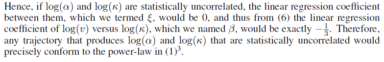
This is the start of the “math”. They say that if Va is constant, equal to some k, then the solution is V = kC^(-1/3), that is all. If Va is constant, you get exactly the 1/3 power law. If D is not constant, you don’t get the exact power law.
I think my favorite narrative is the one where he says he is the guy who barely passed high-school math, but has uncovered an error of “high-powered” researchers…
I mean, the amount of stupid shit that comes from his mouth…
I mean, it is really impossible to discuss anything scientific with a person who cannot admit they were wrong. It is like he has a physical switch that does not allow him to do that - he will confabulate a story where he is still right, even if it means changing the meaning of words, or having obvious logical contradictions, or denying he said things that he definitely said (written proof) (he didn’t mean it).
The problem I have is that I like Bill’s PCT, but I really dislike Rick’s PCT - it is sloppy, inconsistent, and just plain stupid at times. And Rick has a whole bunch of publications that he says are using PCT, but are mostly nonsense. I would rather not be associated with that shit, so I don’t cite his papers, unless I’m writing something to oppose them.
But, you know, he was there first, so I’m just going to use “Control Theory” instead of PCT, I think. That’s what it comes down to. And put him on “ignore” on this forum.
RM: Yes, I think it might be worth it to figure out why this particular side effect occurs. Given the level of misunderstanding of PCT on this site I think it might be worth spending some time on it.
Fine! But you should also figure out why it sometimes occurs and sometimes not. And when it occurs it can have also other power coefficient than 1/3. Your OVB does not answer this. I claims that it occurs always with 1/3 even when it empirically does not occur.
RM: While x and y are 2 df of planar movement, velocity (V) and curvature (C) are not. That’s because V and C (or R) are functions of both x and y see equations 2 and 3 in Marken & Shaffer (2017).
But think: A turn (as a minimal part of curvature) happens when the relationship between the velocities of x and y components of the movement changes. For example x accelerates and y either accelerates less, or keeps constant velocity, or accelerates more, or the same in another way around. Now because x and y are 2 df of planar movement, you cannot predict the change of the velocity of one component from the change of the velocity of the other component. That is why in just the same curvature the total velocity can freely decelerate, remain constant, or accelerate. From the independence of x and y velocities follows the independence of the total velocity and the curvature, no matter what you equations seem to say.
About the equations [V = R1∕3 * D1∕3]; [Width * Height = Area]; [Perimeter = Width + Height]; and also that of the angular speed could be added here [A = C * V], you said: “All these equations are equivalent. They would all be linear if you take the log of both sides in the equations for V and Area.” The first sentence is simply true depending on what you mean here with equivalence of different equations, but they are all similar so that the left side and right side are equivalent: There is always the same value both side when the variables are instantiated and calculations made. So the relationships between the sides are linear even without taking the logs, aren’t they?..
RM: No. Only the equation for P = H + W is linear.
Here is something strange. The value of the Area of an rectangle is always exactly the same as Width times Height. What you mean by saying that it is not linear. (This probably not an important question in relation to our discussion topic, but I just don’t understand.)
And if the equations above are equivalent then there must also prevail a necessary mathematical relationship between the height and with of all possible rectangles. Do you think so? If you think so, then what is the power coefficient of that relationship?
RM: In A = H * W the power coefficient of H is 1 and the power coefficient of W is 1. The equation can be written A = H^1*W^1. The same is true for H and W in P = H + W and for C and V in A = C * V.
Aah! You think that the A = H * W sets or unveils a mathematical relationship between A and W so that there is a linear negative correlation between them, don’t you? But that is true only if the area is constant. If the areas of the rectangles may freely change then that correlation will vanish. Similarly IF affine velocity remains constant THEN there is 1/3 power relationship between velocity and curvature. But if affine velocity may freely change then there is no power relationship or it has a different coefficient.
RM: …There is no law against using regression analysis to confirm a mathematical relationship between variables. And in our case, that use of regression had enormous scientific value because it showed that when you do a regression on only a subset of the variables (V and R) involved in a mathematical relationship that involves those variables and one other (D) your result will deviate from the true relationship between the included two by an amount that is proportional to the covariance between the included and omitted predictor. This is a scientifically important finding because it confirms the PCT explanation of the observed behavior.
A regression analysis which gives exactly the same result from any random data is as valuable as a stopped watch! The result may describe the data by change like the stopped watch shows right time twice a day.
In Marken & Schaffer 2018 you say that:
“[T]he movement trajectories of some physical systems, such as the orbits of the planets, do not follow the 1/3 or 2/3 power law, a fact that we confirmed for ourselves.”
“We also found that the power law is no more obligatory for biological systems than it is for physical systems”
“whether a trajectory is produced by a biological or physical system, a regression analysis based on Eqs. 3 or 4 always finds that the “true” power coefficient for the relationship between the speed and curvature of the movement trajectory is 1/3 (for R versus V) or 2/3 (for C versus A), with an R2 value of 1.0 in both cases”.
So you have admitted yourself that your OVB method gives fabricated results that do not fit – have nothing to do – with the empirical data from which they are calculated!
BTW. How would you proceed if you had a large data of different rectangles and you wanted to know how their widths correlate with their heights?
I think I have read Maoz et al pretty carefully. And while the formulas in our papers differ somewhat in terms of notation, they are exactly equivalent in terms of their meaning. I actually presented this comparison earlier but I guess you may not have seen it. And I suppose you won’t see it here since you are ignoring me. But I will present it again for others who might be interested.
The most obvious equivalence between Marken & Shaffer (M&S) and Maoz et al (Maoz) is in terms of their equations relating velocity, curvature and affine velocity. These are equation (9) in M&S and equation (5) in Maoz:
The only difference between these equations, besides the names of the variables, is that M&S use R as the measure of curvature while Maoz use C, (which they call kappa). Since C = 1/R, their coefficient for the curvature term is -1/3 while ours is 1/3. [The time variable, (t), in equation (5) is actually irrelevant since the regression analysis treats the variables as random variables.]
M&S and Maoz then derive the same implication from equations (9) and (5), respectively. This is shown in the equivalence of equation (12) in M&S and equation (6) in Maoz, as shown here:
These are the equations that give the value of the power coefficient (beta’.obs for M&S, beta for Maoz) that will be observed when log (C) (or log (R)) is regressed on log (V) while log (affine velocity) (log (D) in M&S, and log(alpha) in Maoz) is omitted from the regression.
The equivalence of equations (12) and (6) is important because both are derived using what M&S called Omitted Variable Bias (OVB) analysis. Both show that the observed power coefficient in a regression of log (C) on log (V), omitting log (affine velocity), will be biased from the mathematical value, -1/3, by an amount equal to delta in equation (12) and equal to eta/3 in equation (6) .
The equivalence of M&S equation (12) and Maoz equation (6) requires, therefore, that we see that delta in (12) is equal to eta/3 in (6). This equality can be seen by looking at equation (11) in M&S:
Note that beta.omit is the coefficient of the omitted variable, log (affine velocity), in the “power law” regression of log (C) on log (V). It’s value is 1/3. And the quantity Cov(I,O)/Var(I) is equivalent to eta in equation (6). So equation (12) can be re-written in the form of equation (6); they are the same equation.
This shows that M&S and Maoz did exactly the same OVB analysis. And they come to the same conclusion based on it: A regression of log (C) on log (V), omitting log (affine velocity) will result in a power coefficient that will deviate from - 1/3 to the extent that log (C) correlates with the omitted variable, log (affine velocity); the smaller the correlation between log (C) and log (affine velocity), the closer the power coefficient will be to -1/3.
Actually, it was Pollick & Sapiro who said that. Maoz et al made a more general observation, as follows:
This is a more general statement because, while it’s true there will be zero correlation between affine velocity (D) and C when affine velocity is constant, zero correlation will also happen if D is not constant but the covariance between D and C is 0. But, of course, 0 correlation between D and C happens only for very special movements (like a perfect ellipse, where D is constant). But the correlation between D and C is typically rather low and, as Maoz et al note:
In other words, the chances of doing a regression of log (C) on log (V) and not finding a power coefficient fairly close to -1/3 are small. Indeed, for their Monte Carlo simulations Maoz et al found that the average power coefficient was -.28 with an average R^2 of .57.
So the only difference between the analyses of M&S and Maoz et al is in their conclusions based on their OVB analyses. M&S conclude that the “power law” is an irrelevant side effect of control and the reason researchers typically see a power coefficient for human movement in the range between -.2 and -.4 is because of the mathematical dependence of log(V) on log (C) and (log (affine velocity).
On the other hand, Maoz et al conclude that the -1/3 power law is a true invariant of human movement but that the finding of a 1/3 power coefficient could be a spurious result if it was based on data that was not properly filtered to remove high frequency noise components that would artificially reduce the correlation between log (C) and log (affine velocity).
Actually, my (and Maoz et al’s) OVB analysis ( I explained the equivalence in an earlier post) explains exactly why the -1/3 power law sometimes occurs and sometimes not. And I think your claim would be a little tough to test but maybe you could explain how I could test it.
I don’t have the time or energy to answer the rest of your post now.
RM: Yes, I think it might be worth it to figure out why this particular side effect occurs. Given the level of misunderstanding of PCT on this site I think it might be worth spending some time on it.
Fine! But you should also figure out why it sometimes occurs and sometimes not. And when it occurs it can have also other power coefficient than 1/3. Your OVB does not answer this. I claims that it occurs always with 1/3 even when it empirically does not occur.
Actually, my (and Maoz et al’s) OVB analysis ( I explained the equivalence in an earlier post) explains exactly why the -1/3 power law sometimes occurs and sometimes not. And I think you claim would be a little tough to test but maybe you could explain how I could test it.
I don’t have the time or energy to answer the rest of your post now.
Oh, that is right, there are two equations in common, by bad. They don’t call it OVB, because they are not omitting a variable from the analysis.
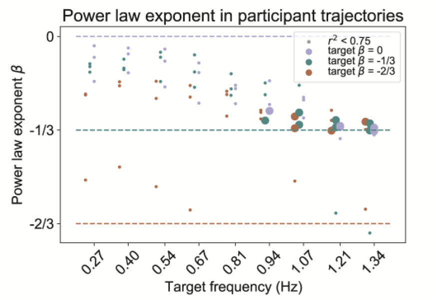
If you take random data, as they do, you get relatively high r2. Also, if data is corrupted by noise. Guard from that by smoothing the trajectories, and only take high r2 (> 0.6) to mean an acceptable power law.
If you take real data from human movement, you get a lot of non-power law movements, especially at lower speeds. From my paper:
The mathematical dependence of three variables has NOTHING to do with the mathematical dependence of two variables.
The questions are:
do humans really slow down in curves in ‘natural movement’ or it is a statistical artifact?
If they do - why? What models can we use to explain human movement?
You (M&S) have two contradictory conclusions - that the power law is a statistical artifact and that it is a side effect of control of something else. Both cannot be true at the same time.
Those conclusions are not contradictory and I’ll explain why. I’ll start by noting that the term “power law” is quite fuzzy. It can refer to the approximately -1/3 power relationship that is often found when curvature is regressed on the velocity of a movement. But it can also refer to the fact that the best fitting relationship between curvature and velocity is typically a power function, even if the power coefficient is not particularly close to -1/3.
I believe the observed relationship between curvature and velocity is considered “real” if the fit of a power function to movement data, measured as R^2, is greater than some value, like .67. Not all movements that are fit by a power function with an R^2 >.67 have a power coefficient of -1/3. Indeed, power coefficients for “real” power laws can deviate considerably from -1/3. So calling the -1/3 power relationship between curvature and velocity a “law” is something of an overstatement. It’s more of an approximation than a law.
I call the power relationship between curvature and velocity – regardless of the value of the power coefficient and R^2 of the fit – an irrelevant side effect of control because there is nothing in the control process that produces curved movements that is designed to produce a power relationship between these variables. The power relationship is, therefore, irrelevant to the control process that produces curved movement in the same sense that the air flow changes around your arm when it is moved are irrelevant to the processes that produced the movement.
The whole statistical artifact business is aimed at explaining why this irrelevant side effect of curved movement – the power relationship between curvature and velocity – is often found, by simple regression analysis, to have a coefficient that is close to -1/3. The explanation is provided by M&S and Maoz et al 's OVB analysis that shows why this happens.
It happens because the actual mathematical power relationship between curvature (C) and velocity (V) has a coefficient of -1/3 but this exact value will only be found by a regression of log (C) on log (V) if the correlation between log (C) and log (affine velocity) – the variable not included in the analysis – is 0.0. However, a value close to -1/3 will typically be found because movements where there is a high correlation between log (C) and log (affine velocity) – which would cause the observed value of the power coefficient to deviate considerably from -1/3 – are quite rare.
So, to summarize:
The observed power relationship between C and V is shown to be an irrelevant side effect of control by the fact that this power relationship is found in the behavior of a control model that accurately mimics the actual movement behavior but contains no provision for producing that power relationship.
The fact that the power relationship between C and V is usually found to have a power coefficient close to -1/3 plus or minus 1/10 is explained by the equations of OVB analysis as presented in M&S and Maoz et al.