Functions and variables and diagrams, oh my!

[JohnGraham]

Continuing the discussion from Question About Feedback Functions:

Moved as per Luk’s suggestion

---

Well now I am very confused

@rsmarken

The thing that makes it tough is that the variable qi, which is shown as being out in the environment, is the SAME variable as p, which is inside the system.

I can see that p and qi can have the same magnitude - or at least the same value, if units are chosen appropriately - but you seem to be implying they have the same identity ( a distinction I am still trying to get my head around). I thought it was pretty important that they are conceptually distinct. (I was starting to think CV most commonly refers to qi - but then see below).

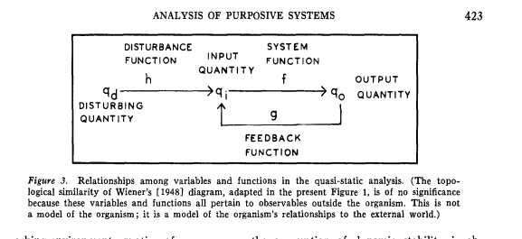
Incidentally I wonder if Powers 1978 is an important early use of the exact term “feedback function” - (in its, phew, unambiguously mathematical sense. Pretty clearly it maps directly onto B:CP’s Environment Function):

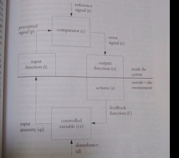
… and then I checked in Tim Carey and Margaret Carey’s RTP Intervention Processes and found this explanation (p120)

A tenet of PCT is that, almost always, the state of particular environmental conditions correlates highly with the state of an individual’s perceptions. So we label environmental conditions that correlate highly with controlled perceptions (p) as controlled variables (cv)

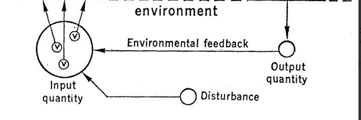
A different diagram once more
So here it looks like CV is conceptually distinct from qi. And as Tim and Margaret also call ‘p’ the ‘controlled perceptual variable’, we’re a hairs-breadth from relabelling CV as Controlled Environmental Variable or Corresponding Environmental Variable. Because it’s ‘p’ that the organism is actually controlling, isn’t it?

Is qi conceptually distinct from CV? Did Bill use the term CV , and that other phrase being used, ‘feedback path’?

Edited to add: Ah, just got how this from the 1973 diagram you posted might help - maybe.

[bnhpct]

@rsmarken

The thing that makes it tough is that the variable qi, which is shown as being out in the environment, is the SAME variable as p, which is inside the system. Both qi and p are a function of environmental variables.

No. If you have an empirical hard science, qi is a quantity measured by the investigator who is studying the behavior of the subject. The value of p is inferred from it in an empirically based model.

On the other hand, if you confound the model with that which is modeled, then qi=p by definition.

@rsmarken

Of course, qo and p are not exactly the same due to noise in the perceptual neural net that computes p, so p = qi + noise. But this noise represents only about 2% of the variance in p so it has little effect on evaluating the accuracy of control models.

This is only handwaving unless you have actually measured p. For which of your models or demos have you measured p?

@rsmarken

The main effect on the accuracy of control models is how accurately you have identified qi, which requires correctly identifying the controlled perceptual variable, p

You can identify the controlled variable, p, the perceptual signal inside the subject, only inferentially. By the TCV you determine that your controlled variable p corresponds to the subject’s controlled variable p. In the TCV, you disturb your own perception from what you think is the subject’s reference value by means of your own outputs affecting a population of perceptible physical variables {v_1, v_2, ‥, v_n} which affect your intensity sensors, although typically you as investigator are controlling a higher-level perception originating in those intensity inputs; and you perceive and ideally measure outputs by the subject affecting that population of physical variables such that your controlled perception is restored to what you posited as the subject’s reference value for it. This is a very good empirical basis for the inference, but it is an inference nonetheless. What you have identified is your own perception of that population of perceptible physical variables {v_1, v_2, ‥, v_n} which you are both affecting. The TCV is a textbook case of the simplest form of collective control, conflict, gently initiated so that the subject can overcome it easily. It is the same, functionally, as letting the opponent win the tug of war or the arm wrestling. Two levels could model it.

But what you identify in physical fact is the population of perceptible physical variables {v_1, v_2, ‥, v_n} which affect your intensity sensors and the subject’s intensity sensors, and which are affected equally by your outputs and the subject’s outputs. This is what is called the CEV or CCEV, which you (as the investigator) demonstrate to be actually present in the environment precisely because both you and the subject are demonstratedly affecting it at the same time. This is a disciplined form of the social method by which living things test and demonstrate the reality of what they perceive to be real. It is the essence of scientific method, and the reason for publishing demonstrations which any properly trained colleague can replicate and possibly falsify. All of science is inferential, as any competent scientist will tell you. Engineers, medical practitioners, and non-scientists generally, require the findings of science to be authoritative. But I digress. I’m sure you know this. I want to avoid any appearance of demeaning your knowledge or intelligence.

The model is not that which is modeled. You are far from the only scientist who confounds the model with that which is modeled. For one critique, see

Lissack, M. R., & Richardson, K. A. (2001). When Modeling Social Systems, Models ≠ the Modeled: Reacting to Wolfram’s A New Kind of Science. Emergence, 3(4), 95–111. https://doi.org/10.1207/S15327000EM0304_7

[EetuP]

I thought that (according the theory) p (inside the subject) is (or should be) an analog of the qi (outside the subject, in the environment). So p and qi cannot be the same variable, even though their variabilities behave similarly.

Eetu

Lähetetty Outlook for Android

[rsmarken]

@JohnGraham

Continuing the discussion from Question About Feedback Functions:

Moved as per Luk’s suggestion

---

Good idea.

@JohnGraham

Well now I am very confused

@rsmarken

The thing that makes it tough is that the variable qi, which is shown as being out in the environment, is the SAME variable as p, which is inside the system.

I can see that p and qi can have the same magnitude - or at least the same value, if units are chosen appropriately but you seem to be implying they have the same identity ( a distinction I am still trying to get my head around).

The identity of qi and p is defined by the formula that defines them. If qi and p are the area of the rectangle then both are defined as h * w; if qi and p are the perimeter of the rectangle then both are defined as 2*(h + w). What’s confusing you (and clearly you are not alone in your confusion!) is the fact that qi has identity (for example, you know what the area of the rectangle “looks like”) while p is (in theory) a neural signal that varies only in magnitude; it seems to have no identity.

But in PCT p does have an identity and it is defined by the perceptual function that produced it. The magnitude of p is an analog of variations in the perceptual variable that is defined by the perceptual function. When you are controlling the area of the rectangle, you define qi as h * w and, in theory, the perceptual function defines p as h * w.

But, you say, p doesn’t “look like” qi, so how can I say that p = qi? One is a neural signal and the other is a pattern of light out there in the world? I’ll try to explain it in terms of an inanimate control system, the cruise control system in your car. This system has a perceptual function that converts the rotation of the wheels of your car into an electrical signal, p.v, which is a perception of velocity. The perceptual function is:

p.v = 2 * pi * r *f

where pi is 3.14159, r is the wheel radius and f is wheel revolutions per second. So p.v is an electrical analog of velocity in units of distance/duration making p.v is an electrical (perceptual) analog of the controlled variable, qi.v, which happens to be

qi.v = 2 * pi * r *f

So, even in a non-living control system, p = qi.

But perhaps you are still confused because, unlike the cruise control system, you don’t see just electrical signals when you control the area or perimeter of the rectangle. What you are running into here is the “hard problem” of consciousness, the problem being “Why the f**k does the world look like this when I know it’s just electrical signals in my brain”! And I have a not so great answer to that question: That’s the way the world looks when you ARE the neural signals (and perceptual functions) involved in dealing with the ourside world.

But the best way to understand that qi = p in a control system is to do some modeling of control systems. And you might also take a look at “receptive field cells” to get an idea of how perception works, in PCT and in physiology.

@JohnGraham

I thought it was pretty important that they [qi and p] are conceptually distinct.

Yes, qi is the “objectively observed” controlled variable (objectively observed using some version of the test for the controlled variable) and p is its theoretical counterpart that is used in models of behavior.

[quote=“JohnGraham, post:1, topic:16275, full:true”]
… and then I checked in Tim Carey and Margaret Carey’s RTP Intervention Processes and found this explanation (p120)

A tenet of PCT is that, almost always, the state of particular environmental conditions correlates highly with the state of an individual’s perceptions. So we label environmental conditions that correlate highly with controlled perceptions (p) as controlled variables (cv)

Tim is one of only 3 people who I would tell anyone to go to if they wanted to know what PCT was about. And he is by far the best writer on things PCT. Nevertheless, I judge this to be a rather awkward way of making the distinction between cv (qi) and p. But I think it’s OK as long as “environmental conditions” are understood to be conditions (like the area or perimeter of a rectangle) that are functions of sensory (and, ultimately, environmental) variables.

@JohnGraham

So here it looks like CV is conceptually distinct from qi.

No, there are just two concepts, CV (or qi) and p. Bill has also used “Controlled Quantity (CQ)” and “Input Variable” for qi and when he used CQ for qi he has used CV for p. Clearly, the distinction between CV and p (whatever you call them) is difficult to communicate, even for the extremely lucid developer of PCT, but it becomes completely non-confusing when you code up a working control system simulation of some control behavior, like tracking.

@JohnGraham

And as Tim and Margaret also call ‘p’ the ‘controlled perceptual variable’, we’re a hairs-breadth from relabelling CV as Controlled Environmental Variable or Corresponding Environmental Variable. Because it’s ‘p’ that the organism is actually controlling, isn’t it?

I never liked the term Controlled Environmental Variable because it implies that what we control are entities in the environment when, in fact, we control functions of environmental variables.

@JohnGraham

Is qi conceptually distinct from CV? Did Bill use the term CV , and that other phrase being used, ‘feedback path’?

No, qi and CV refer to the same thing; the aspect (or function) of the environment that is controlled. Again, I know that all of this can be difficult but once you do some modeling of control behavior it all becomes perfectly clear. I say this because I struggled with these terminological difficulties until I started to do modeling of actual behavior. It’s the best teacher, at least for would-be scientific psychologists.

[rsmarken]

@bnhpct

@rsmarken

The thing that makes it tough is that the variable qi, which is shown as being out in the environment, is the SAME variable as p, which is inside the system. Both qi and p are a function of environmental variables.

No. If you have an empirical hard science, qi is a quantity measured by the investigator who is studying the behavior of the subject. The value of p is inferred from it in an empirically based model.

What I meant (and what should have been clear from context) is that qi and p are the SAME mathematically, not materially. See my cruise control example in my reply to John.

@bnhpct

On the other hand, if you confound the model with that which is modeled, then qi=p by definition.

No, the mathematical equivalence of qi and p still exists when you don’t confound the model with what is modeled, as I don’t.

@bnhpct

@rsmarken

Of course, qo and p are not exactly the same due to noise in the perceptual neural net that computes p, so p = qi + noise. But this noise represents only about 2% of the variance in p so it has little effect on evaluating the accuracy of control models.

This is only handwaving unless you have actually measured p. For which of your models or demos have you measured p?

This one (see p. 10)

@bnhpct

@rsmarken

The main effect on the accuracy of control models is how accurately you have identified qi, which requires correctly identifying the controlled perceptual variable, p

You can identify the controlled variable, p, the perceptual signal inside the subject, only inferentially. By the TCV you determine that your controlled variable p corresponds to the subject’s controlled variable p.

No, you determine whether your hypothesized controlled variable corresponds to the subject’s controlled variable. The hypothesized CV is not controlled by the experimenter in the TCV; it is simply disturbed by the experimenter (or natural events).

@bnhpct

In the TCV, you disturb your own perception from what you think is the subject’s reference value

No, you don’t need to guess what the subect’s reference level might be. Indeed, the test works even if the subect’s reference is randomly varying, as it is in my mind reading demo of the TCV.

@bnhpct

The TCV is a textbook case of the simplest form of collective control, conflict, gently initiated so that the subject can overcome it easily. It is the same, functionally, as letting the opponent win the tug of war or the arm wrestling. Two levels could model it.

There is no conflict in the TCV. You don’t understand the difference between a passive and active disturbance. The disturbances in the TCV are passive; the disturbances in a conflict are active, inasmuch as they are produced by the outputs of other control systems.

I think that’s enough error correction for one post!

[rsmarken]

Hi Eetu

@EetuP

I thought that (according the theory) p (inside the subject) is (or should be) an analog of the qi (outside the subject, in the environment). So p and qi cannot be the same variable, even though their variabilities behave similarly.

Again, they are the same mathematically.

[JohnGraham]

@rsmarken

So p.v is an electrical analog of velocity in units of distance/duration

Just for clarity, p itself is in something like impulses per second, isn’t it? With units/conversion factor chosen so that k.i = 1 signal unit per physical unit. It’s the choice of units that makes p=q.i, correct?

[rsmarken]

No, it’s because p is the same function of physical variables as q.i. The physical variables are the lengths of the horizontal (h) and vertical (v) lines of pixels on the screen. The function that defines both q.i and p when q.i is the area of the rectangle made by the lines is h * v. The function that defines both q.i and p when q.i is the perimeter of the rectangle is 2 * (h + v).

The same is true of a speedometer and an accelerometer. The physical variable that is the basis of the perception of both velocity (by the speedometer) and acceleration (by the accelerometer) is wheel rotation rate (f). The function that defines both q.i and p when q.i is velocity (v) is 2 * pi * r * f. The function that defines both q.i and p when q.i is acceleration is dv/dt.

Have you tried the “What is size” demo? If you do, try to see that the different perceptions you can control – area and perimeter – are constructed by your perceptual systems from the SAME constituents – the same lines on the screen – using different construction “blueprints” (the different equations that define area and perimeter).

Best, Rick

[JohnGraham]

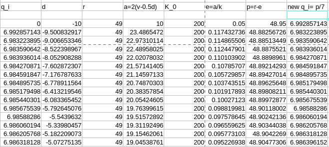
Well, the good news is you’ve “made me” fire up my spreadsheet.

Ok. Your demos are all great. Invaluable resources.

My physics tutor brain (undergrad minor only in some past century) won’t rest unless, as in B:CP, p = k.i*q.i, with p in signal units, q.i in physical units, and k.i in signal units per physical unit. It has to be that way for the units analysis to work.

So if q.i. = 2h + 2v
Then it must be that p= k(2h+2v). It’s just that k=1

Only then can it relax and let my maths tutor brain (undergrad major only in same distant century) ignore all of that and say fine, p=q.i, let’s look at the spreadsheet/ code.

If I have this wrong then my brain shall be the locus of some major reorganisation .

I’m given some confidence by Bill writing in “The Basics of Control Theory” in Introduction to Modern Psychology p53:

In a real person, the perceptual signal is (presumably) a neural signal [note1: “Measured in terms of frequency-impulses per second, for example”] representing some equivalent measure of the externally observable variable. We always can pick units for measuring neural frequencies which make the conversion factor in the input function equal to 1, as in “one Nervous System Unit (NSU per inch”[note 2:"If a 1-inch displacement results in a signal of 137 impulses per second, we just call 137 impulses per second 1 NSU, and draw the markings on our meters accordingly].

So it seems like k.i. = 1 by convention and obvious convenience. Note to self, if I’m ever tempted to create a schism within PCT, I’ll start a sect where k.i. = 7.

I tried it in the spreadsheet I made of that chapter (souped up with varying disturbance) - and it seems to work fine as long as I remember to make r equal to k.i times the target q.i

I’m still quite a distance from knowing exactly what this spreadsheet even means - so thank you for taking your time on this foundational stuff with me. As a maths student I never quite figured out how numbers and what passes for reality are supposed to fit together, so this question seems quite important.

[EetuP]

I don’t think that expression “being mathematically same” and “being an analog” have exactly the same meaning.
A variable a is an analog of a variable b if (b = 2 x a) but I wouldn’t say that a and b are mathematically same.

Eetu

Lähetetty Outlook for Android

[wmansell]

Agreed.

[rsmarken]

@JohnGraham

Ok. Your demos are all great. Invaluable resources.

Well, finally I get agreement on something;-) Thanks!

@JohnGraham

My physics tutor brain (undergrad minor only in some past century) won’t rest unless, as in B:CP, p = k.i*q.i, with p in signal units, q.i in physical units, and k.i in signal units per physical unit. It has to be that way for the units analysis to work.

Bill was a physics BS, as was my gradutate advisor. But dimensional analysis won’t help you here. What is needed is an understanding of the relationship between theory and obsevation. I wish I myself had thought of this sooner but today it struck me that this whole debate about whether q.i = p is ridiculous because p is a theoretical entity which Bill proposed to explain the existence of the observed phenomenon of controlled variables – qi. So p was proposed to equal qi.

You can see this in the segement you quoted from Bill’s “The Basics of Control Theory” in Introduction to Modern Psychology p53. I’ll just highlight the part relevant to the issue of whether qi = p:

In a real person, the perceptual signal is (presumably) a neural signal representing some equivalent measure of the externally observable variable.

Saying the perceptual signal (p) is presumably a neural signal highlights the fact that p is theoretical and that it was proposed as an equivalent measure of the externally observable variable – the controlled variable qi. In other words p is the theoretical equivalent of qi, or qi = p.

What creates a problem is that qi looks like a scalar variable. But, in fact, qi is typically a complex function of environmental variables, x.i. So qi = f(x.1,x.2…x.n). Since p is quivalent to qi (in theory) then for all controlled variables, qi, it’s proposed (in theory) that p = f(x.1,x.2…x.n) as well.

In the model, f() is presumed to be a perceptual function in the control system under study. In the observer, f() is either the same perceptual function in the observer as in the system under study or, it is the function of a device, such as a speedometer or accelerometer, that is designed to perceive (measure) that variable.

In PCT, it is presumed that there are different f()'s for different controlled variables. One of the most significant theoretical proposals of PCT is that the different controlled variables are controlled at different levels of a hierarchy of control systems in the organism and that the perceptions controlled at these different levels are of different types (intensity, sensation, cofiguration…principles, system concepts). These different types of perceptions are computed by neural nets that represent differnet types of percepual functions, f().

I built a spreadsheet model of a three level hierarchy of control systems, with control systems at each level controlling a different type of perceptual variable. A write up about the spreadsheet and the spreadsheet itself can be found here.I think if you learn what’s going on in this spreadsheet model you will have come a long way toward really understanding PCT.

[JohnGraham]

@EetuP

A variable a is an analog of a variable b if (b = 2 x a) but I wouldn’t say that a and b are mathematically same.

I did not know this meaning of ‘analog’, thank you Eetu!

And thank you also Rick @rsmarken - looks like I have plenty of homework to do.

[Lukasz20]

A few observations on dimensional analysis, environmental physics, and PCT modelling

I have followed this exchange with considerable interest. The discussion of whether the environmental quantity q_i and perception p are “the same variable”, and whether dimensional analysis is useful, raises a practical question: how do we specify a model so that its physical meaning and computational results are unambiguous?

I would like to approach this from the perspective of control engineering and dynamical systems.

1. Dimensional analysis is not a formality

John Graham is right to raise the question of the coefficient k_i and consistency of units. When we relate quantities with different physical dimensions, we need a transformation that accounts for that difference. Equality of numerical values alone does not establish the physical identity of the quantities.

The loss of Mars Climate Orbiter in 1999 is a useful warning against overlooking units. Thruster impulse data were supplied in pound-force seconds (lbf·s), while the navigation software expected newton-seconds (N·s). [1]

This example requires an important qualification: the two units have the same physical dimension but different scales. Dimensional analysis alone would not have detected the error. Unit conventions and conversions also needed to be checked. A model must address both.

In a simple PCT model, we distinguish:

• q_i — an environmental quantity, such as position, force, or voltage;
• p — an internal perceptual signal, with a specified representation and scale;
• p = f(q_i) — the input function relating the two.

For a linear input function, we write p = k_i · q_i, with the coefficient satisfying the dimensional relation [k_i] = [p] / [q_i].

Writing p = q_i can be a valid simplification when the scales or normalisation are appropriately defined. I use this assumption in my own calibration example. It does not, however, eliminate the distinction between the role of the environmental quantity and that of the perceptual signal. An identity input function is a specific modelling assumption that should be made explicit.

The system’s action changes the environment and, through the input function, affects perception. Preserving these relationships in the model makes it clear what reaches the comparator and how action affects the measured quantity.

2. From a spreadsheet to a numerical experiment with explicit checks

A spreadsheet is a valuable tool for exploring a control loop. A correctly implemented method with a fixed time step can also produce reliable research results.

The requirements for computational reliability remain the same, regardless of the tool:

• Numerical error control. An excessively large step can distort the dynamics or introduce artificial instability. We need to check whether reducing the step or tightening the tolerances materially changes the result.
• Explicit handling of discontinuities. Values immediately before and after an event must be distinguished, and discontinuities must be accounted for during integration. This applies to adaptive solvers as well.
• Explicit limits on action. If we are investigating actuator saturation or the accumulation of integral state while the output is saturated (integrator windup), these effects must be represented in the model. Changing the solver does not remove them. [2]
• Reproducibility. Another researcher should receive the equations, parameters, initial conditions, disturbance protocol, and numerical settings needed to check the result.

RK45 helps control local error by adapting the step size, but it does not guarantee that the model is correct or that the method is suitable for every system. [3]

Automating these checks and making the complete experiment available are my reasons for developing a dedicated research environment.

3. A practical example: Livia — PCT Research Laboratory

Over the past few days, I have brought a working prototype with a browser interface into operation:

Livia — PCT Research Laboratory

I am developing it so that researchers can define and test models without writing their own solvers, while keeping assumptions explicit and computations open to inspection.

The current implementation includes:

• A compiler using restricted expression trees and dimensional analysis. It checks the declared dimensions of signals and derivatives. A dimensional inconsistency in an equation or comparator causes the model to be rejected. This checks dimensional consistency; it does not automatically establish physical validity.
• Distinct roles within the loop. The engine distinguishes the environmental quantity q, perception p, comparator input pc, reference signal r, and error e = r - pc. This makes it possible, for example, to hold the signal available to the comparator constant while continuing to measure the actual modelled perception.
• Matched experimental conditions. Normal operation (live), held output (output_held), and held comparator input (feedback_held) are each computed both with and without the disturbance. These interventions allow the roles of action and current perceptual feedback in the model’s response to be examined.
• Event handling and accuracy checks. The engine splits integration at scheduled event boundaries, records values on both sides, and compares trajectories with calculations made under tighter solver settings.
• Metrics and export. The researcher receives measures including a disturbance suppression ratio and recovery time, together with a package containing the model, protocol, data, and code for repeating the calculations outside the browser.

In a simple integral-controller calibration example, the functioning loop compensates for the disturbance, while compensation disappears under either ablation. The exported trajectory was checked against the known analytical solution; the maximum difference was approximately 2.76 × 10⁻⁹. This verifies a specific numerical case. It is neither an empirical validation of a psychological mechanism nor a validation of the entire tool.

Livia remains a prototype under active development. Before opening it for testing, I am refining package verification, the criteria for confirming reproduction, and report readability. Access is deliberately restricted while I prepare the Zenodo deposit and documentation.

4. A proposed next step

I believe PCT would benefit from accessible tools that let us translate conceptual differences into explicit differences in equations and then test their consequences.

I would welcome suggestions for models, disturbances, and edge cases on which to test Livia, particularly cases with known solutions or clearly specified predictions. I am equally interested in cases where the tool should report a limitation, an unresolved result, or failure to meet a criterion.

My aim is for a researcher to be able to share a complete experiment alongside the diagram and interpretation: assumptions, equations, disturbances, results, and a way to reproduce them. That is the standard I am working towards with this project.

Luk

Technical references

1. NASA, Mars Climate Orbiter: mission overview and Phase II investigation report.
2. MathWorks, Anti-Windup Control Using PID Controller Block.
3. SciPy, solve_ivp documentation.

[JohnGraham]

Thanks Luk - as you can probably surmise, some of what you write is beyond my current capabilities and purposes, but the first part reassures me my excursion into the “elusive obvious” has not been entirely ridiculous! You’ve also raised a point I might later tease out, for this thread, in terms of the ambiguity/interpretation of the word “function”.

One possibility for a spinoff thread: in your paragraph “Explicit limits on action” starts to appear the kind of terminology which might be less familiar to many readers of PCT, and this to me is the point where you and Rick often seem to start talking past each other. Your very helpful footnote points to the concept of a PID controller. It is striking that the diagram linked to there, and also the block diagram of a “PID controller” on the relevant Wikipedia page, looks unlike a PCT control loop, in a way I feel I might better understand once I’ve mastered Powers’ 1978 “Quantitative Analysis” paper. Perhaps if so inclined you or someone else familiar with the issues could at your leisure expound upon/discuss the relationship between something like a PID controller, and PCT.

Best regards,
John

[rsmarken]

@JohnGraham

One possibility for a spinoff thread: in your paragraph “Explicit limits on action” starts to appear the kind of terminology which might be less familiar to many readers of PCT, and this to me is the point where you and Rick often seem to start talking past each other. Your very helpful footnote points to the concept of a PID controller. It is striking that the diagram linked to there, and also the block diagram of a “PID controller” on the relevant Wikipedia page, looks unlike a PCT control loop, in a way I feel I might better understand once I’ve mastered Powers’ 1978 “Quantitative Analysis” paper. Perhaps if so inclined you or someone else familiar with the issues could at your leisure expound upon/discuss the relationship between something like a PID controller, and PCT.

I think this is a great idea. I suggest you start a spinoff thread where we can discuss the difference between the PID and PCT diagram of a controller. Maybe call it “A Tale of Two Circuities”. I’ll chime in after I hear what one or two others think.

[wmansell]

Rick, the word in Bill’s quote you missed out in your elaboration of his quote is ‘representing’…

[wmansell]

A dimmer switch dial covaries near perfectly with the luminessence of the light filament, but it is not the same thing. And in the real world, different disturbances affect each.

[Lukasz20]

I’m very much in favour of a separate thread. John’s question prompted me to revisit a few things myself, particularly which parts of the diagrams correspond and how terms such as “input” and “output” are being used. I’d be interested to hear others’ perspectives and then contribute what I’ve found.

Luk

[JohnGraham]

@Lukasz20

I’m very much in favour of a separate thread.

Edit: here we go: PID controllers etc. and PCT