[From Bill Powers (2009.11.15/0116 MDT)]
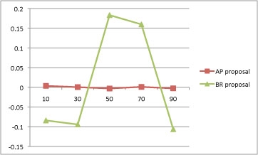
Rick Marken (2009.11.13.1620) –
While I await Martin’s
description of the difference between the variables controlled by the AP
and BR models, I’ve gone to the trouble of creating my own spreadsheet
with the Ariely data and wrote up a quick version of my model (which I
think is the BR model which Martin found to do so much more poorly than
the AR model). I see that Bill did the same. My model still needs work
but I would like to get it into a form where I can compare it to the AR
model. So I would like to see what your AR model looks like, Martin.
My model, too, needs work – I realized last night that it doesn’t make
any sense the way I wrote it because I forgot the idea I had previously
come up with, which is probably close to yours.
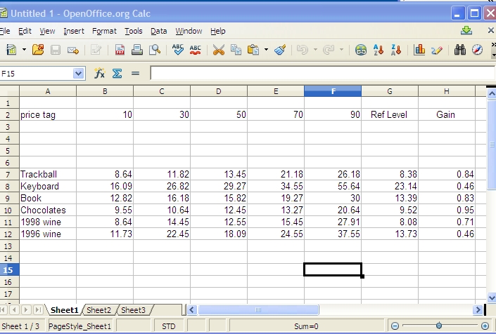
Look at the first column of data. There are three cases (bold-faced)
where the SS# is lower than the average of the binned “bid” by
the population of subjects in that column. In the other 27 cases, the
mean bid number is lower than the mean SS#. Note that until further
notice I’m treating this table of population data as if it applies to
some average individual. Later I’ll correct that.
Range of last two digits of SS number
Products
00-19 20-39 40-59
60-79
80-99 Correlations
Cordless
Trackball
8.64 11.82
13.45 21.18
26.18
0.42
Cordless
Keyboard
16.09 26.82
29.27 34.55
55.64
0.52
Design
Book
12.82 16.18
15.82 19.27
30.00
0.32
Chocolates
9.55 10.64
12.45 13.27
20.64
0.42
1998
Wine
8.64 14.45
12.55 15 45
27.91
0.33
1996
Wine
11.73 22.45
18.09 24.55
37.55
0.33If the “subjects” (i.e. a fictitious average subject) are
thinking of the SS# as a price tag, then they clearly would purchase
those three items at the asked price because they’re willing to pay more
than the asked price. Notice the term “asked price.” This table
begins to make sense if we think of it as the first step in each of 30
bargaining sessions. The SS# is the opening “asked” price,
which the subject sees before deciding what to do. The “bid”,
in all but those three cases, is the amount the subject offers in return
to end that round of bargaining.
The three bold-faced bids would never be made; if the offering price is
already lower than the amount the subject would bid, the bargaining would
end there and the transaction would occur unless the bid and asked prices
were sealed before the end of each round. And then there would have to be
some prior agreement about what to do if the asked price is less than the
bid – split the difference or whatever. The bargaining would still end
there.
In the other 27 cases, the item would not be purchased because the bid
price is less than the (assumed) asked price, under this way of
conceptualizing the situation.
If this is seen as a bargaining session, in the 27 “live” cases
the next step would be for the seller to lower the asked price and/or the
bidder to increase the bid. If the bidder does not increase the bid and
the seller does not lower the price there is no deal and the item is not
purchased.
A deal is made when the seller lowers the asked price to or below the
buyer’s reference level for the price. So how do we determine the buyer’s
reference level? It might change on every round, so we need a way to
determine its apparent value after every round. Start by considering the
two differences between bid and asked price (from the first two columns,
in this case)
Asked price Mean Bid price
Difference, Bid - Asked
···
10.00
8.64
-1.36
30.00
11.82
-18.18
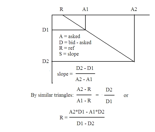
The question now is, “At what asked price would the difference go to
zero?” Here is a plot of a straight-line relationship between the
asked price A and the difference D between bid and asked, bid - asked,
with an easy geometric solution for the reference level and the
slope:
![Emacs!]()
For the first two entries in the first row of data we have
slope = (-18.18 - (-1.36))/(30 - 10) = 16.82/20
= -0.841
ref = (30*-1.36 - 10*-18.18)/(-1.36 + 18.18)
= (-40.8 +
181.8)/16.82
  = 141/ 16.82

  = 8.383
Check: diff = -0.841*(asked - 8.383):
asked = 10; diff = -0.841*1.62 = -1.36
asked = 30; diff = 0.841* 21.617 = -18.18
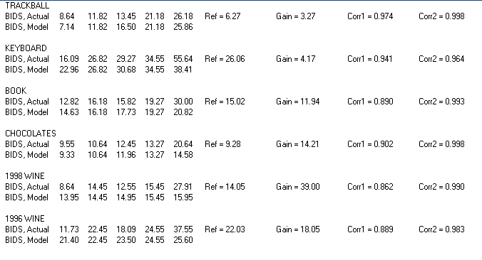
Rick, I’m sure you can set this up as a spreadsheet a lot faster than I
can. To get rid of the extra step of computing the difference, use
diff = bid - asked,
so the equation becomes
bid = (k + 1)asked - kref
where k and ref are determined as in the graphic above.
You can do this for any two columns.
==========================================================================
To set this up as a simulation, clearly you have to have two parties: a
seller and a bidder, both adjusting their respective asked and bid prices
on each round. And just as clearly, you have to treat each individual and
each trial as a separate case; the population bid and asked prices are
meaningless for individuals, they are of interest only to a seller
Runkeling the data to take advantage of the average properties of a
population.
Runkeling: do not go gentle into that good night; rage, rage against the
dying of the light.
This model should be applied to each experimental run, and each person in
the population has to make repeated bids as the asked price is changed.
The reference levels and slopes have to be calculated for each
individual, not for the averaged measures over the population.
The Arielly data is clearly insufficient to allow any conclusions to be
drawn about individuals; it would be like ranking chess teams by having
each member of one team make one move against just one member of the
other team, then trying to evaluate how good the average move was. I
assume that each participant in the experiment made just one bid on each
item against the last two digits of his own SS#.
It would be somewhat interesting to give one person repeated trials while
the asked price is varied randomly. But the most interesting case would
be to have pairs of subjects playing buyer and seller seeing whether they
can reach a deal on various items, and calculating the reference level
and slope for each person after each round. Another situation would be an
auction with a video camera to record successive bids for the same item
by each person. We’d have to work out the equations for that
model.
We can be quite sure of one thing. The SS# does not “leak” into
the bid number, somehow. That was just a stab in the dark. The meaning of
these data depends entirely on how the subject conceived the situation.
This is not a simple cause-effect phenomenon. We have to try out various
models: price tag, bid-asked, whatever else you can come up with. Each
proposal for how the subjects perceived the situation will lead to a
slightly different model. And of the utmost importance, we should NOT use
population data. If we want to say anything about the population, we
should first determine the parameters for each individuals, then find
their means and distributions.
Best,
Bill P.