What happened to CSGnet?

[Bill_Powers1]

[From Bill Powers (2009.11.18.1221 MDT)]

Martin Taylor 2009.11.18.10.36] –

It’s interesting that you have a
problem with your control analysis that is analogous to my problem with
the (probably) artifactual uniformity of the mean error averaged across
objects within SS# bands. I have no answer to either, at the
moment.

I think the explanation is clear now. A straight line of data points will
correlate with another straight line even though the slopes are
different, which is why correlations are useless for fitting models to
data. I’ve now changed the program so it adjusts the reference level and
gain to get the best values of gain and reference by minimizing the RMS
difference between the real and modeled “output” variable,
which is just Asked - Bid price. The optimized values of gain and
reference are used for both the bids and the outputs. The optimization is
repeated 10 times, going back and forth between gain and reference
adjustment. That achieves perhaps a 10% reduction in RMS error relative
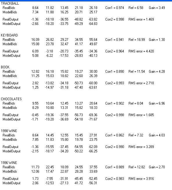
to a single iteration. Here is the table of results (it’s a jpeg graphic,
a cropped screen shot, also attached):

As you can see, the RMS error between RealOutput and ModelOutput is
reasonably small; for the Keyboard row, which has the largest RMS error,
it;'s about 11% of the maximum output (4.4 out of 40). The correlations
(Corr2) range from 0.983 (worst) to 0.998 (best). I’ve attached the final
version of the AriellyUn Unit, where all the calculations are shown. It
just produces the table above, so is of interest only to programmers who
can read the pascal code. Not commented much, I’m afraid. I’m about
burned out on this for the time being.

Best,

Bill P.

AriellyUn2.pas (6.22 KB)

[rsmarken]

[From Rick Marken (2009.11.18.1320)]

Bill Powers (2009.11.18.1221 MDT)–

Martin Taylor 2009.11.18.10.36] –

It’s interesting that you have a
problem with your control analysis that is analogous to my problem with
the (probably) artifactual uniformity of the mean error averaged across
objects within SS# bands. I have no answer to either, at the
moment.

I think the explanation is clear now. A straight line of data points will
correlate with another straight line even though the slopes are
different, which is why correlations are useless for fitting models to
data.

I was going to mention that but I wanted to hold my options open for presenting more economic correlations (which don’t involve model fitting;-). Yes, the correlation number is unaffected by a linear transformation of the variables being correlated. So the correlation between X and Y is the same as the correlation between aX+b and a1Y+b1. RMS is the only way to go when testing models.

Best

Rick

···

–
Richard S. Marken PhD
rsmarken@gmail.com
www.mindreadings.com

[rsmarken]

[From Rick Marken (2009.11.19.2030)]

Bill Powers (2009.11.17.0621 MDT)]

The control model I’m using is

R R = Reference signal

v

—>Comp—

G G = gain

      >

      v

B<----------O O = output

^ B = bid

A A = asked (SS#)

The output is not observable since it’s whatever the person does
internally to keep the bid from being completely determined by the asked
price, as in a store where there is no choice. So I have had to use the
controlled variable, B, as the basis for computing gain and reference
level. For really tight control systems this usually exaggerates small
errors and gives a poor fit. fortunately, the gains are relatively low
here.

The control equations are

(1) B = O + A

(2) O = G(R - B)

Solving for B we get

A + GR

(3) B = --------

1 + G

Just for the heck of it, I tried a model that assumed that the bids were the outputs (O) and that the CV was O - A. In my model the CV (O-A) is equivalent to B (O+A) in your model but in my model O is the observed bid while in yours O is an imagined bid and B is the obserbed one. In my model, the data (observed bids) are considered the outputs (O) that keep B under control. Solving for O in my model gives the equation for predicting the observed bids:

G (R + A)

   O =  --------------

1 + G

I compared this model to yours and there appears to be no difference in the predictions. I fit the models using a “manual” hill-climbing (or, better, valley-finding) technique where I adjusted the values of G, R and A to minimize the RMS error between actual and predicted bids, the predicted bids being B in your case and O in mine. The minimum RMS error for your model was 2.7 bid units; for my model it was 2.6. I think that if I had used a real mathematical minimization algorithm the model fits would have been exactly equivalent, which leads me to believe that the models are mathematically equivalent. But these models are different in terms of how they map to behavior. In your model, the observed bids are the controlled variable; in my model the observed bids are outputs that keep the controlled variable – O-A – under control. There must be a way to distinguish these models experimentally. Any ideas?

By the way, I’m attaching the spreadsheet so you can see what I did and, of course, correct any errors (there always are errors).

Best

Rick

Ariely.xls (26 KB)

···

–
Richard S. Marken PhD
rsmarken@gmail.com

www.mindreadings.com

[MartinT]

[Martin Taylor 2009.11.20.00.06]

[Martin Taylor 2009.11.18.10.36]

It's interesting that you have a problem with your control analysis that is analogous to my problem with the (probably) artifactual uniformity of the mean error averaged across objects within SS# bands. I have no answer to either, at the moment.

I do now. I realized that what I was doing to get the scaling function was actually equivalent to taking the geometric mean of the bids across all the objects and then finding the multiplier that would make all the geometric means the same across SS#s, even though the procedure looked different on its face. Geometric means usually aren't too very different from arithmetic means, so in retrospect it's not very surprising that the arithmetic means across SS#s were so similar.

It's always humbling to make mistakes that in retrospect are so obvious

Martin

[Bill_Powers1]

[From Rick Marken
(2009.11.19.2030)]

RM: Just for the heck of it, I tried a model that assumed that the
bids were the outputs (O) and that the CV was O - A. In my model the CV
(O-A) is equivalent to B (O+A) in your model but in my model O is the
observed bid while in yours O is an imagined bid and B is the obserbed
one. In my model, the data (observed bids) are considered the outputs (O)
that keep B under control.

As near as I can translate that, this is the diagram you mean (please
correct if it’s wrong):

R R = Reference signal

v

—>Comp—

G G = gain

      >

      v

   [CV]

(B-A)<--------B [output = B = observed bids]

Since A, the asked price, is a given of the data (SS#, not adjustable),
this is equivalent to

R R = Reference signal

v

—>Comp—

G G = gain

      >

•    v
  

   [CV] 

(B)<---------B [B = observed bids]

^

A

I can’t make sense of this, because it says (B) = B - A. So I must not be
understanding what you said.

Solving for O in my model gives the equation for predicting the
observed bids:

G (R + A)

   O =  --------------

1 + G

How about modifying my diagram above so it shows what you mean, then
writing the two system equations so I can see them, and finally solving
them first for the output and then for the controlled variable? Then
maybe I’ll be able to understand.

Best,

Bill P.

···

At 08:29 PM 11/19/2009 -0800, you wrote:

[Bill_Powers1]

[From Bill Powers (2009.11.20.0650 MDT)]

Martin Taylor 2009.11.20.00.06 --

MT: I realized that what I was doing to get the scaling function was actually equivalent to taking the geometric mean of the bids across all the objects and then finding the multiplier that would make all the geometric means the same across SS#s, even though the procedure looked different on its face.

BP: I really must be slowed down today because I can't make sense of that, either. Are you and Rick ganging up on me?

The "geometric mean of the bids across all the objects" means to me a total of 30 bids, 5 bids on each object and 6 objects. To make sure, I looked up the meaning of "geometric mean" on the Web and found "the n-th root of the product of n numbers." I can't imagine what that would signify. Are you sure you didn't intend to say the six geometric means of the bids for each object? Is that what "all the geometric means across SS#s" means?

MT: Geometric means usually aren't too very different from arithmetic means

BP: Really? I guess you're right for the first row of bids: arithmetic mean = 16.25, geometric mean = 15.0. whaddaya know?

Am I to guess that you were averaging the logs of all the bids? The antilog of the average log would produce the geometric mean, wouldn't it?

MT: so in retrospect it's not very surprising that the arithmetic means across SS#s were so similar.

BP: It's hard to understand what you mean when you're communicating only some unknown fraction of it. If I understand your shorthand, you're talking about the arithmetic means down a column of the data for one SS#, and the similarity to which you refer is not a similarity from one column to another, but a similarity between the arithmetic and geometric means within any one column. I don't see what that has to do with the two plots you showed, but perhaps that's moot now.

Does this mean you now have different plots?

Best,

Bill P.

[rsmarken]

[From Rick Marken (2009.11.20.1200)]

Rick Marken
(2009.11.19.2030)

RM: Just for the heck of it, I tried a model that assumed that the
bids were the outputs (O) and that the CV was O - A. In my model the CV
(O-A) is equivalent to B (O+A) in your model but in my model O is the
observed bid while in yours O is an imagined bid and B is the obserbed
one. In my model, the data (observed bids) are considered the outputs (O)
that keep B under control.

As near as I can translate that, this is the diagram you mean (please
correct if it’s wrong):

R R = Reference signal

v

—>Comp—

G G = gain

      >

      v

[CV]
(B-A)<--------B [output = B = observed bids]

This is correct.

Since A, the asked price, is a given of the data (SS#, not adjustable),
this is equivalent to

R R = Reference signal

v

—>Comp—

G G = gain

      >

•    v
  

[CV]
(B)<---------B [B = observed bids]

^

A

Yes. Exactly. What you call [B = observed bids] is what I still call O.

I can’t make sense of this, because it says (B) = B - A. So I must not be
understanding what you said.

It’s a notational problem. I’m trying to keep you notation but change the variables that correspond to the observed bid. In both of out models B is the controlled variable. In your model B = O + A and you thought of O as an imaginary output and B as the observed bid. So you solved for B to predict the observed data. In my model, B = O - A and O corresponds to the observed bid, which is combined with A to produce the hypothesized controlled perception, B. So I solved for O (rather than B) to predict the observed data.

How about modifying my diagram above so it shows what you mean, then
writing the two system equations so I can see them, and finally solving
them first for the output and then for the controlled variable? Then
maybe I’ll be able to understand.

My system equations

B = O-A
O= G(R-B)

solving for O

O = G(R - (O-A))
=GR - G(O-A
…

          G(R+A)

(1) O = -----------
(1 + G)

I leave solving for the controlled variable as an exercise;-)

Formula (1) is what I use in the spreadsheet to predict the data values.

Maybe this would have been less confusing if I had just used B to refer to the observed bids and change your B to CV so the system equations would be

CV = B-A

B= G(R-CV)

In that case, the equation (1) would be the same except that O would be B.

          G(R+A)

(1a) B = -----------

          (1 + G)

Best

Rick

···

On Fri, Nov 20, 2009 at 5:49 AM, Bill Powers powers_w@frontier.net wrote:

Richard S. Marken PhD
rsmarken@gmail.com
www.mindreadings.com

[MartinT]

Bill Powers wrote:
[Martin Taylor 2009.11.20.17.02]

[From Bill Powers (2009.11.20.0650 MDT)]

Martin Taylor 2009.11.20.00.06 --

MT: Geometric means usually aren't too very different from arithmetic means

BP: Really? I guess you're right for the first row of bids: arithmetic mean = 16.25, geometric mean = 15.0. whaddaya know?

Am I to guess that you were averaging the logs of all the bids? The antilog of the average log would produce the geometric mean, wouldn't it?

Yes, but I hadn't noticed it until a couple of days ago, in the same way you hadn't noticed that any two linear trends are perfectly correlated. Blind spot

MT: so in retrospect it's not very surprising that the arithmetic means across SS#s were so similar.

BP: It's hard to understand what you mean when you're communicating only some unknown fraction of it.

Sorry, I didn't want to repeat myself too often. I thought you already knew the plot I referred to.

If I understand your shorthand, you're talking about the arithmetic means down a column of the data for one SS#, and the similarity to which you refer is not a similarity from one column to another, but a similarity between the arithmetic and geometric means within any one column. I don't see what that has to do with the two plots you showed, but perhaps that's moot now.

What it has to do with the plot is that you "took your hat off" to me for finding a regularity in the data, when that regularity turned out to be just that there isn't much difference between geometric and arithmetic means. I don't think it's moot now, at all. If there's a question as to which of several possible variables is being controlled, then the one whose computed values best match the data is the one likely to be nearest the truth. You don't have to know the details of the control system for that, even though it's much more satisfactory if you do have a control structure that implements the proposed control.

Does this mean you now have different plots?

No. Since analysis of my proposal (modification of the perceived scale of the bid numbers by the SS#) is shown to be dependent on the average bid across objects, it is not feasible to use that analysis to get a trend across SS#s. We know that the linear trend is wrong, but we have no principled way of choosing another. All I do have is the standard deviations of the fits, which I reported earlier.

Martin

[Bill_Powers1]

[From Bill Powers (2009.11.20.1550 MDT)]

Rick Marken (2009.11.20.1200) –

BP earlier: Since A, the asked
price, is a given of the data (SS#, not adjustable), this is equivalent
to

R R = Reference signal

v
—>Comp—

G G = gain

      >

•    v
  

[CV]
(B)<---------B [B = observed bids]
^

A

RM: Yes. Exactly. What you call [B = observed bids] is what I still call
O.

BP: All right, then your diagram is this:

R R = Reference signal

v

—>Comp—

G G = gain

      >

      v

B<----------O

^

A

As you can see, B, the observed bid, is now the controlled variable, O is
the output of the control system, and A is a disturbance applied to
B.

Here is my diagram from the first post containing it that I sent on
11.17.0621. Can you see any difference? I can’t.

R R = Reference signal

v

—>Comp—

G G = gain

      >

      v

B<----------O O = output

^ B = bid

A A = asked (SS#)

Here are your system equations:

RM: My system equations

B = O-A

O= G(R-B)

solving for O

O = G(R - (O-A))

=GR - G(O-A

…

G(R+A)

(1) O = -----------

(1 + G)

BP: … and here are mine:

The control equations
are

(1) B = O + A

(2) O = G(R - B)

Solving for B we get

A + GR

(3) B = --------

1 + G

Notice that I solved for B, whereas you solved for O. Also, you said B =
O - A instead of O + A, which means you have to enter A as a negative
number. Solving my equations for O, I get

G(R - A)

    O = ------------

1 + G

Other than the minus sign, that seems identical to your solution, no? It
looks as if we have come up with identical equations and solutions except
for one sign.

I’m trying to keep your notation
but change the variables that correspond to the observed bid. In both of
our models B is the controlled variable. In your model B = O + A and you
thought of O as an imaginary output and B as the observed
bid.

Maybe this is the problem: B is not the observed bid from the data, but
the bid that the model would produce, which will be different from the
observed bid until you adjust the gain and reference level properly. B in
the above diagrams is clearly the controlled input variable. O is an
output affecting the controlled variable. Have you matched the output of
the control system to the observed bids?

I’ve just re-examnined your spread-sheet model and indeed that is what
has happened. Your gains are all less than 1, so the output O matches the
observed values of B. In my latest version, the gains are all about 10
times as great, and model B matches the observed values of real B. If you
calculate the values of B for your model, you’ll see that they are all
much less than the observed values. Try matching B to the data by
adjusting the parameters and you should see that B(model) now matches
B(real) and the gain is higher. My latest values for B are slightly
different because I’ve added an automatic matching program that uses all
five bid values in adjusting G and R. Your manual matching should give
about the same values if you go back and forth between G and R a few
times.

I’m still not satisfied with my arrangement of the model because it
doesn’t really show how the Asked price affects the imagined value of B.
There’s just an arrow saying that the effect takes place. If I figure out
something better than that I’ll post it.

Best,

Bill P.